Showing posts with label svg. Show all posts

Thursday, December 11, 2014

Out of Nowhere–Explore Text on a Path

I had not really stopped to think of this until I listened to this The Web Ahead podcast with Sara Soueidan.  What is really interesting about the tech world is how experts can seemingly pop up out of nowhere and become the authority on a topic.  In the podcast, this was the case with the interviewee Sara Soueidan.  We can find a similar example in Joni "Bologna" Trythall with SVG.

I find it even more fun when I can incorporate these experts’ content into R.  Let’s animate some text on a path as Joni does in her article "Animating SVG text On A Path", but instead of an arbitrary path, let’s use a line in a plot.

some text on a path

I’ll copy the code below.  Let me know if a tutorial would be helpful.

library(SVGAnnotation)
library(pipeR)
library(htmltools)

# make as basic a line plot as I know how in R
svg = svgPlot(plot(sin(seq(0,pi*3,0.2)),type="l")) %>>%
# extract the XML and use htmlParse
# to overcome namespace confusion and difficulty
saveXML %>>% htmlParse

# with base R plots, we get clues with clip-path attributes
# in this case we know with some inspection
# there will be one g with a clip-path attribute
# and that g will contain our plotted line
getNodeSet(svg,"//g[contains(@clip-path,'url')]//path")[[1]] %>>%
# let's add an id so we can reference this later
( addAttributes( node=., id = "ourline" ) )

# first step in adding text to a path
# make a new text node
textOnPath = newXMLNode("text")
# now the critical part to join the text to the path
addChildren(
textOnPath
, newXMLNode(
"textPath"
,attrs=c( "xlink:href" = "#ourline" ) #our id given above
,"some text on a path" #some very creative saying
)
)

# add our text node to the svg plot
addChildren(
getNodeSet(svg,"//svg")[[1]]
,kids = list(textOnPath)
)
# see if it works by sending to our viewer/browser
getNodeSet(svg,"//svg")[[1]] %>>%
saveXML %>>% HTML %>>% html_print

# let's continue our journey by exploring the startOffset attribute
# startOffset says where on the path to start our text
# what happens if we add startOffset = 30%
getNodeSet(svg, "//textPath")[[1]] %>>%
( addAttributes( node = . , startOffset = "30%" ) )
# find out the effect of startOffset by browsing
getNodeSet(svg,"//svg")[[1]] %>>%
saveXML %>>% HTML %>>% html_print

# for our grand finale we can animate the text
# note: this might not work in your browser, so use Chrome
# add a child animate node with the same attributes as Joni's tutorial
getNodeSet(svg, "//textPath")[[1]] %>>%
(
addChildren(
node = .
, newXMLNode(
"animate"
,attrs = c(
attributeName="startOffset"
,values = "0;0.7;1"
,dur = "8s"
,repeatCount = "indefinite"
,keyTimes = "0;0.2;1"
)
)
)
)
# see the animated text
getNodeSet(svg,"//svg")[[1]] %>>%
saveXML %>>% HTML %>>% html_print(viewer=utils::browseURL)

Tuesday, December 2, 2014

Much Better Animated Paths | Christmas SVG

Just after I made my really ugly animated turkey sketch (see post), I saw this much better set of Christmas icons in the Smashing Magazine Article Freebie Christmas Icon Set from Manuela Langella.  While I still remember how to do this, I thought I would use the same techniques in R using rvest + XML + htmltools to animate the paths with vivus.js.  In the iframe below is the result on the Santa icon.

Code: http://gist.github.com/39394d6e37a7fd878cab#file-code-R

Wednesday, November 26, 2014

Happy Thanksgiving | More Examples of XML + rvest with SVG

I did not intend for this little experiment to become a post, but I think the code builds nicely on the XML + rvest combination (also see yesterday’s post) for working with XML/HTML/SVG documents in R.

It all started when I was playing on my iPhone in the Sketchbook app and drew a really bad turkey.  Even though, the turkey was bad, I thought it would be fun to combine with vivus.js.  However, Sketchbook does not export SVG, so I exported as PDF and imported into Inkscape.  The end result was a still very messy SVG file, so I thought it would be a great test / application of my new skills with rvest + XML. The code opens the SVG, grabs all the path nodes, assembles those into a svg tag with id = "turkey", and then adds a script to use the addDependency for vivus.js.

Happy Thanksgiving to all the US readers out there.

Friday, October 10, 2014

SVG + Javascript Ekholm Decomposition in RStudio Browser

Our topics this week seem unrelated, but in an effort to bridge the two

another random project – make website in R for these SVGs of Portland Vector Bridges
result: Portland Bridges in SVG
code: R to make simple site

Ekholm decomposition

SelectionShare & TimingShare | Masterfully Written by Delightfully Responsive Author
Popular Mutual Funds Decomposed With Ekholm (2014)

Responsive SVG in the browser

Responsive SVG in Your RStudio Browser
SVG + a little extra (d3.js) in RStudio Browser | No Pipes This Time

let’s build a website in R with htmltools to calculate the Ekholm decomposition in Javascript using this nifty simple-statistics.js from the brilliant Tom Macwright.  The result will not be beautiful and I’ll leave out a fancy interactive chart, but that is intentional to reduce the amount of code and dependencies.
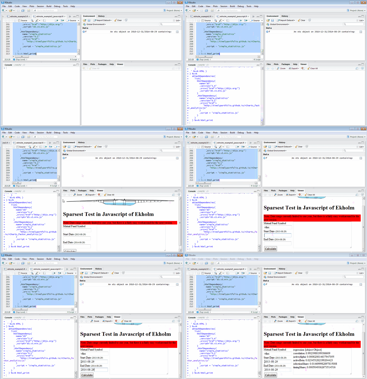
r_ekholm_js

I wonder what I’ll get into next week.

Github Repo

library(htmltools)
library(pipeR)
library(jsonlite)
library(Quandl)
library(xts)

# use Quandl Kenneth French Fama/French factors
# http://www.quandl.com/KFRENCH/FACTORS_D
#f <- Quandl("KFRENCH/FACTORS_D",type = "xts", start_date="2010-12-31") / 100

tagList(
#pull in the bridge to span all the week's topics
#Portland Vector Bridges http://timelyportfolio.github.io/portland_vector_bridges
tags$div( style = "height:15%;width:100%"
,readLines(
"http://timelyportfolio.github.io/portland_vector_bridges/Burnside Bridge.svg"
) %>>% HTML
)
,tags$h1( "Sparsest Test in Javascript of Ekholm")
, tags$div( style = "width:100%"
,tags$div( style = "background-color:red;"
,"Note: Date range currently limited to one year, but there is a fairly easy workaround
for the next version."
)
,tags$div(
style = "display:inline-block; width: 25%;float:left;"
,"Mutual Fund Symbol", tags$input( id = "mfsymbol" )
,tags$br()
,"Start Date "
, tags$span( style="font-size:75%;fill:lightgray", "(2013-08-29)" )
, tags$input( type = "date", id = "stdate" )
,tags$br()
,"End Date"
,tags$span( style="font-size:75%;fill:lightgray", "(2014-08-29)" )
, tags$input( type = "date", id= "enddate" )
,tags$br()
,tags$input(
type="submit", id = "calc", value = "Calculate"
)
,tags$br()
)
, tags$div(style = "display:inline-block;height:100%;width:60%;margin-left:30px"
, tags$textarea(id = "results", style="width:100%; height:150px")
)
)
,tags$script(sprintf(
'

var french = %s;
'
, toJSON(data.frame("Date"=index(f),f)) %>>% HTML
))
,tags$script(
'

function calculateEkholm( data ) { // data in form of x,y or fund-rf, mkt-rf
/* get an error with regression.js
var myReg = regression(
"linear",
data
)
*/

// so use the great simple-statistics library
var myReg = ss.linear_regression().data(data);

//get residuals
var resid = data.map(function(p){return myReg.line()(p[0]) - p[1]});

//regress residuals^2 on (mkt-rf)^2
var myReg2 = ss.linear_regression().data(
data.map(function(d,i){
return [ Math.pow(d[0],2), Math.pow(resid[i],2) ]
})
)
//coefficients ^ 1/2 will give us ActiveAlpha and ActiveBeta
var activeAlpha = Math.pow( myReg2.b(), 0.5 );
var activeBeta = Math.pow( myReg2.m(), 0.5 );

//now do the next step to get ActiveShare and SelectionShare
var selectionShare = Math.pow(activeAlpha, 2 ) / ( ss.variance(data.map(function(d){return d[1]})) * (data.length - 1) / data.length )
var timingShare = Math.pow(activeBeta, 2 ) * ss.mean( data.map(function(d){return Math.pow(d[0],2)}) ) / ( ss.variance(data.map(function(d){return d[1]})) * (data.length - 1) / data.length )

//pass correlation result also
var correlation = ss.sample_correlation(data.map(function(d){return d[0]}),data.map(function(d){return d[1]}));

return {
regression: myReg,
correlation: correlation,
activeAlpha: activeAlpha,
activeBeta: activeBeta,
selectionShare: selectionShare,
timingShare: timingShare
}
}


// thanks https://gist.github.com/fincluster/6145995
function getStock(opts, type, complete) {
var defs = {
desc: false,
baseURL: "http://query.yahooapis.com/v1/public/yql?q=",
query: {
quotes: \'select * from yahoo.finance.quotes where symbol = \"{stock}\" | sort(field=\"{sortBy}\", descending=\"{desc}\")\',
historicaldata: \'select * from yahoo.finance.historicaldata where symbol = \"{stock}\" and startDate = \"{startDate}\" and endDate = \"{endDate}\"\'
},
suffixURL: {
quotes: "&env=store://datatables.org/alltableswithkeys&format=json&callback=?",
historicaldata: "&env=store://datatables.org/alltableswithkeys&format=json"
}
};

opts = opts || {};

if (!opts.stock) {
complete("No stock defined");
return;
}

var query = defs.query[type]
.replace("{stock}", opts.stock)
.replace("{sortBy}", defs.sortBy)
.replace("{desc}", defs.desc)
.replace("{startDate}", opts.startDate)
.replace("{endDate}", opts.endDate)

var url = defs.baseURL + query + (defs.suffixURL[type] || "");

return url;
}


d3.select("#calc").on("click",function(){
calculateFund(
d3.select("#mfsymbol")[0][0].value,
d3.select("#stdate")[0][0].value,
d3.select("#enddate")[0][0].value
)
})

function calculateFund( symbol, startdate, enddate ) {

d3.json(getStock({stock:symbol.toUpperCase(),startDate:startdate,endDate:enddate},"historicaldata"), function(e1,fund){


if( e1 || !fund.query.results ) {
updateResults ( {e1:e1, e2:e2, queryresults: "query problems"} );
} else {
var fund_factor = [];

//manipulate data to join fund with factors
//would be nice to have a xts merge in javascript


// query.results.quote will have the data stripped of meta
// also we will sort date ascending
fund = fund.query.results.quote
.sort(function(a,b){
return d3.ascending(
d3.time.format("%Y-%m-%d").parse(a.Date),
d3.time.format("%Y-%m-%d").parse(b.Date)
)
} );


// now lets go period by period with fund.map
fund.map( function(per, i){
if( i > 0 ) {
var frenchThisPer = french.filter(function(d){return d.Date == per.Date})[0];
fund_factor.push([
//Date: per.Date,
//FundPrice:
per.Adj_Close / fund[ i - 1 ].Adj_Close - 1 - frenchThisPer["RF"],
//Rm_Rf:
+frenchThisPer["Mkt.RF"],
//Rf: +frenchThisPer["RF"]/100
])
}
})

updateResults( calculateEkholm( fund_factor ) );
}

})
}

function updateResults( ekholmCalc ){
var ekhArr = [];
Object.keys(ekholmCalc).map(function(k){
ekhArr.push( [ k,": ", ekholmCalc[k] ].join("") )
})
d3.select("#results").text(ekhArr.join("\\n"))
}
'
%>>% HTML )
) %>>%
attachDependencies(
list(
htmlDependency(
name="d3"
,version="3.4"
,src=c("href"="http://d3js.org/")
,script="d3.v3.min.js"
)
,htmlDependency(
name="simple_statistics"
,version="0.1"
,src=c("href"=
"http://timelyportfolio.github.io/rCharts_factor_analytics/js"
)
,script = "simple_statistics.js"
)
)
) %>>% html_print

Thursday, October 9, 2014

SVG + a little extra (d3.js) in RStudio Browser | No Pipes This Time

I’m guessing here, but yesterday’s post Responsive SVG in Your RStudio Browser might have inspired some “but,…)”s, “yes plus I need”s, “what the %>>% with the pipe”s, etc.  I’ll attempt to address a couple of these in this quick post.

First, if you don’t like pipes, here is the non-piped version of the code.  I also made one change, which assumes that you want the SVG to fill the <div> container.  This is helpful if you think you will only have one plot and nothing else in your HTML.

library(SVGAnnotation)
library(htmltools)

respXML <- function( svg_xml, height = NULL, width = "100%", print = T, ... ){
# svg_xml should be an XML document
library(htmltools)
library(XML)

svg <- structure(
ifelse(
length(getDefaultNamespace(svg_xml)) > 0
,getNodeSet(svg_xml,"//x:svg", "x")
,getNodeSet(svg_xml,"//svg")
)
,class="XMLNodeSet"
)

xmlApply(
svg
,function(s){
a = xmlAttrs(s)
removeAttributes(s)
xmlAttrs(s) <- a[-(1:2)]
xmlAttrs(s) <- c(
style = paste0(
"height:100%;width:100%;"
)
)
}
)

svg <- HTML( saveXML( svg_xml) )

svg <- tags$div(
style = paste(
sprintf('width:%s;',width)
,ifelse(!is.null(height),sprintf('height:%s;',height),"")
)
,svg
)

if(print) html_print(svg)

return( invisible( svg ) )
}


Second, I like it but I’m helpless without my Javascript helper libraries, such as d3.js, Snap.svg, Raphaël, etc.  htmltools makes it fairly easy to attach dependencies.  Let’s add d3.js in this example.


Third, I want to use my helper library to add some script to make something awesome.  I can’t help with the awesome part, but I can show you how to add a little bit of code.  This time we’ll take the simple pan/zoom code from ggplot2 meet d3, and here is the result.  Please understand that this is only 4 lines of Javascript, so the pan/zoom is not nearly as refined as I would expect.


R_svg_d3js


# make our plot here
# since we will need to manipulate to add a g container
# for smoother d3 pan/zoom
sP = respXML(
svgPlot(
dotchart(
t(VADeaths)
, xlim = c(0,100)
, main = "Death Rates in Virginia - 1940"
)
)
, height = "100%"
, print = F
)

# parse the plot html with rvest
sP = html(as.character(sP))
# add a g node to contain the plot
# for smoother d3 pan / zoom
g = newXMLNode("g")
# add the old g to our new g container
addChildren(g, html_nodes(sP,"svg > g"))
# add our new g container to our svg
addChildren(html_nodes(sP,"svg")[[1]],g)

html_print(attachDependencies(
tagList(
# get the div with our modified svg
HTML(saveXML(html_nodes(sP,"div")[[1]]))
, tags$script(
HTML(
'
var g = d3.select("svg > g");
var zoom = d3.behavior.zoom().scaleExtent([1, 8]).on("zoom", zoomed)
g.call(zoom)

function zoomed() {
g.select("g")
.attr(
"transform",
"translate(" + d3.event.translate + ")scale(" + d3.event.scale + ")"
);
}
'

)
)
)
,htmlDependency(
name="d3"
,version="3.0"
,src=c("href"="http://d3js.org/")
,script="d3.v3.js"
)
))

Wednesday, October 8, 2014

Responsive SVG in Your RStudio Browser

For those readers who are unaware, SVG is absolutely amazing, and if you need some convincing see this 2009 paper/talk from David Dailey Why is SVG Going to Be REALLY BIG?  Most R users should be very well acquainted with graphics and plots magically appearing on the screen with certain commands.  These graphics though are rasters, so when you resize, the graphics are re-rendered to scale.  Let’s have a look with a simple plot.

plot(x=1:10,y=1:10,type="b")


R_raster_resize


One of the beauties of SVG is that it will scale without re-rendering.  The old way to create SVG in R was to do something like this which produces an svg file that we can use, adjust, and share.

svg("svgplot.svg")
plot(x=1:10,y=1:10,type="b")
dev.off()

However, the integrated browser window in RStudio combined with the HTML helper tools  from RStudio lets us produce and see SVGs in real-time.  Let’s look again at our simple plot, but this time as an SVG in our RStudio browser window.  We will also use the precocious packages SVGAnnotation and XML from Duncan Temple Lang.


R_svg_1


But where is the magic resizability ?


This is where we will use some help from


Sara Soueidan - Understanding SVG Coordinate Systems & Transformations (Part 1) – The viewport, viewBox, & preserveAspectRatio


Dudley Storey - Make SVG Responsive


We can make a simple function to help us change the attributes and style to get a fancy responsive SVG real-time.

#even better make it responsive
#use this post as a guide
#http://demosthenes.info/blog/744/Make-SVG-Responsive
respXML <- function( svg_xml, height = NULL, width = "100%", print = T, ... ){
# svg_xml should be an XML document
library(htmltools)
library(pipeR)
library(XML)

tags$div(
style = paste(
sprintf('width:%s;',width)
,ifelse(!is.null(height),sprintf('height:%s;',height),"")
,"display: inline-block;"
,"position: relative;"
,"padding-bottom: 100%;"
,"vertical-align: middle;"
,"overflow: hidden;"
)
, ...
,svg_xml %>>%
(~svg ~
structure(ifelse(
length(getDefaultNamespace(svg)) > 0
,getNodeSet(svg,"//x:svg", "x")
,getNodeSet(svg,"//svg")
),class="XMLNodeSet") %>>%
xmlApply(
function(s){
a = xmlAttrs(s)
removeAttributes(s)
xmlAttrs(s) <- a[-(1:2)]
xmlAttrs(s) <- c(
style = paste0(
#"height:100%;width:100%;"
"display: inline-block;"
#post says use these but will not fit viewer
#,"position: absolute;"
#,"top: 0;"
#,"left: 0;"
)
#,preserveAspectRatio="xMidYMid meet"
)
}
)
) %>>%
saveXML %>>%
HTML
) %>>%
( ~ if(print) html_print(.) ) %>>%
( return( invisible( . ) ) )

Let’s test our fancy new function.


R_svg_2


That’s more like it.  Let’s abandon the animated GIFs and embed a SVG below (copied/pasted straight from R into this post).  Resize your browser and test the result.


Actually, it appears I lied. The SVG does not resize like it would outside the Blogger container.  See http://bl.ocks.org/timelyportfolio/raw/560e50e437d4bb1b9142/ for the SVG in a standalone document for resizing.

# example using dotchart documentation
# in R graphics package
# ?graphics::dotchart
svgPlot(
dotchart(
t(VADeaths)
, xlim = c(0,100)
, main = "Death Rates in Virginia - 1940"
)
) %>>%
respXML