Statistics of Drawdown–paper and post

Thank so much to Patrick Burns’ post Variability in maximum drawdown.  He starts with “Maximum drawdown is blazingly variable,” which I say is why money management is so blazingly difficult.  After spending a lot of time thinking about his post and trying to replicate the referenced paper

Casati, Alessandro, About the Statistics of the Maximum Drawdown in Financial Time Series (May 1, 2012). Available at SSRN: http://ssrn.com/abstract=2049584 or http://dx.doi.org/10.2139/ssrn.2049584

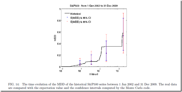
I think that the cumulative statistics, both total return and drawdown, fit well with the comment “The pictures imply that the maximum drawdown could have been pretty much anything.” Here is one of the figures that leads to this conclusion, and the predicted confidence interval from 20% to 90% is incredibly wide and not all that helpful.  If someone was willing to pay me for the bet that over the next 1,000 days, the S&P 500 or really any equity index drawdown falls between 20% and 90%, I would be happy to take that bet, and I would not need sophisticated statistical techniques to give me that insight.

Although I do not replicate the paper exactly with the most obvious difference that I use monthly returns 1950-May 2012 rather than daily returns 2002-2009, we can evaluate both return and drawdown through density plots with multiple distribution methods.  I limited my simulation to 10,000 samples so that I would not be up all night, but 10,000 is sufficient to show that over 62 years, both cumulative return and max drawdown can be virtually anything and both are “blazingly variable.”  I wonder how this would compare with life with sickness/death as drawdown and age of death as cumulative return.

From TimelyPortfolio

From TimelyPortfolio

To be fair, let’s annualize the cumulative returns (actually probably better to do over 5 to 20 year periods).

From TimelyPortfolio

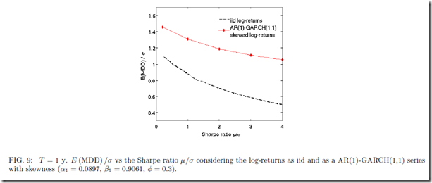
Independent of the outcome, I really enjoyed the paper’s Figures 8, 9, and 10 getting me one step closer to the question posed in my post Is Drawdown the Biggest Determinant of System Success?

We do see a relationship between return and drawdown.

From TimelyPortfolio

If nothing else, I was delighted to see a discussion of the often ignored drawdown statistic, which is the key to every investment decision I make.

R code from GIST:

Is Drawdown the Biggest Determinant of System Success?

In all my system development, I still have not been able to determine what universal underlying conditions significantly improve a system’s chances of outperforming buy-and-hold.  Also, I have found very little discussion, so maybe R with some help from ttrTests can help answer my question of when I should just go buy-and-hold (a very pleasant situation for a money manager).  Starting in this business in 1998, I have often said that I dream of a day when I can just buy and hold similar to Japan stocks 1980-1990, US stocks 1990-2000, and US bonds 1982-now.

Those who follow my blog or know me already understand my obsession with drawdown, but that obsession focuses more on client/manager psychology (Investing for the Long Run) rather than drawdown’s effects on tactical systems.  I do not understand the industry’s focus on standard deviation.  I have never had a client call me or even worse fire me because my standard deviation has increased.  I know the argument is that higher standard deviations lead to higher drawdown, but as I show later in the post, this does not seem to be the case.

Clients call me or fire me because they have lost money, so if I can minimize the frequency, amplitude, and duration of drawdowns, then I can help/guide the client and reduce the worry, which is one main reason why they are paying me.  Also, though I think that focusing on minimizing drawdown can meaningfully increase the chances of achieving their long term return objectives (Drawdown Control Can Also Determine Ending Wealth and Confidence, Ending Equity, and What I Can Do as the Money Manager), which is even more likely the reason why clients pay me.

How nice would it be if drawdown also determines an objective system’s success?  To start the testing I thought I would use the fine work of David St. John on ttrTests (ttrTests 4th and Final Test) to get 100,000 bootstrapped samples from monthly S&P 500 data to examine drawdown, standard deviation, skewness, and compound returns on buy-and-hold versus a Mebane Faber 10-month moving average system.  Since I am so biased, I will let you determine the significance of drawdown on the results.

From TimelyPortfolio

From TimelyPortfolio

Here is where I get some confidence in my belief higher standard deviation does not necessarily cause worse drawdowns. However, it is interesting that higher standard deviation has as high a correlation as drawdown with system out(under)performance (bottom right).

From TimelyPortfolio

R code from GIST:

ttrTests This is a Test Test 3:Data Snoopy

THIS IS NOT INVESTMENT ADVICE.  IT IS JUST AN EXAMPLE AND WILL LIKELY LOSE LOTS OF MONEY IF YOU PURSUE WHAT IS DISCUSSED.  READER IS RESPONSIBLE FOR THEIR OWN GAINS OR LOSSES.  IF YOU ARE AN UNLIKELY WINNER, I WOULD LOVE TO HEAR YOUR STORY.

When we are deciding on a quantitative system to guide our investments, we have multiple choices all fraught with potential luck:  investment choice, system type, system, timeframe, system parameter or parameters, and money management.  To really gain some confidence in the persistence of your choices, I believe each choice should be as rigorously tested as possible.  http://math.uic.edu/~dstjohn/thesis.pdf, http://ageconsearch.umn.edu/bitstream/19039/1/cp05pa01.pdf, and http://www.ssc.wisc.edu/~bhansen/718/White2000.pdf all offer very good discussion of some of the tests.  My posts ttrTests This is a Test--Test 1 and Test 2, ttrTests: Its Great Thesis and Incredible Potential, and ttrTests Experimentation offer a simple application of the much-less-than-simple statistical tests.

I will apply the dataSnoop test with Hansen’s test for Superior Predictive Ability (SPA) to check for luck in the parameter choice of my simple CUD indicator.

I hate to do this, but I cannot think of an easy way to describe the output of the dataSnoop test, so I hope you will read http://math.uic.edu/~dstjohn/thesis.pdf pages 51-57.  Here is the paper’s description of the tests when applied to a MACD system. 

http://math.uic.edu/~dstjohn/thesis.pdf page 55

p-values for my CUD indicator are not so good.

CUD: Observed P-values for Means 'l', 'c', and 'u' respectively: 0.4 0.4 0.97

The observed values from the test are plotted below.

From TimelyPortfolio

R code (click to download from Google Docs):

 

#let's define our silly countupdown function
#as a sample of a custom ttr rule
CUD <- function(x,params=50,...) {
	#CUD takes the n-period sum of 1 (up days) and -1 (down days)
	temp <- ifelse(runSum(ifelse(ROC(x,1,type="discrete") > 0,1,-1),params)>=0,1,0)
	#replace NA with 0 at beginning of period
	temp[is.na(temp)] <- 0
	temp
}   require(ttrTests)
require(quantmod)
require(lattice)
require(reshape2)
require(PerformanceAnalytics)   #defaults functions is overridden by ggplot2 and plyr if loaded
#and will cause problems if you want to use ttrTests concurrently   tckrs <- c("GSPC","RUT","N225","GDAXI","DJUBS")   #use 1 or GSPC but adjust however you would like
i=1
getSymbols(paste("^",tckrs[i],sep=""),from="1896-01-01",to=Sys.Date())
test_price <- as.vector(get(tckrs[i])[,4])   #run dataSnoop to test for luck
#by checking all parameters across multiple bootstrap samples
#this takes a long time, so for experimenting change bSamples to
#something smaller than 100
#if you are planning to use this for commercial purposes
#make sure you see the warning in the documentation
#on Dr. Halbert White's patent and his paper
#http://www.ssc.wisc.edu/~bhansen/718/White2000.pdf   #don't get me started on patents of this sort   #crit can be "sharpe", "return", or "adjust"
#will choose "sharpe" but feel free to try them all
snoop <- dataSnoop(x=test_price, ttr = CUD, start = 20, nSteps = 30, stepSize = 10,
	bSamples=100, crit="sharpe",
	restrict = FALSE, burn = 0, short = FALSE, condition = NULL,
	silent = TRUE, TC = 0.001, loud = TRUE, alpha = 0.025,
	begin = 1, percent = 1, file = "", benchmark = "hold")   #make output slightly more usable with some naming
#believe I got this right
names(snoop) <- c("details","V1","V2",
	"V3","p1.for.l","p2.for.c","p3.for.u")   #jpeg(filename="dataSnoop values.jpg",
	quality=100,width=6.25, height = 6.25,  units="in",res=96)
plot(snoop$V3,
	type="l", col=2,
	main="ttrTests dataSnoop V1,V2,and V3 on CUD",
	xlab="Bootstrap Sample", ylab="Values")
points(snoop$V2, type="l", col=3)
points(snoop$V1, col=4)
legend("topright",legend=c("V1","V2","V3"),col=c(4,3,2),pch=19,lty=1)
#dev.off()

Created by Pretty R at inside-R.org

ttrTests This is a Test--Test 1 and Test 2

Just to remind everyone, THIS IS NOT INVESTMENT ADVICE AND ANY ACTIONS TAKEN BASED ON THIS DISCUSSION WILL PROBABLY RESULT IN SIGNIFICANT LOSSES.

We had fun with the ttrTests package in two previous posts ttrTests: Its Great Thesis and Incredible Potential and ttrTests Experimentation.  Let’s actually run some real tests on the basic CUD indicator introduced in A Quantstrat to Build On Part 6.  We will start by using paramStats to test multiple parameters.

From TimelyPortfolio

After we find the best parameter, we will test with returnStats the actual returns using the best parameter for the CUD indicator versus a buy-and-hold approach.

From TimelyPortfolio

Finally, we will try to apply some statistical rigidity to the process by using 100 bootstrapped samples to test the best parameter on out-of-sample data. As always, please let me know your thoughts.

From TimelyPortfolio

From TimelyPortfolio

From TimelyPortfolio

R code (click to download from Google Docs):

#let's define our silly countupdown function
#as a sample of a custom ttr rule
CUD <- function(x,params=50,...) {
	#CUD takes the n-period sum of 1 (up days) and -1 (down days)
	temp <- ifelse(runSum(ifelse(ROC(x,1,type="discrete") > 0,1,-1),params)>=0,1,0)
	#replace NA with 0 at beginning of period
	temp[is.na(temp)] <- 0
	temp
}   require(ttrTests)
require(quantmod)
require(lattice)
require(reshape2)
require(PerformanceAnalytics)   #defaults functions is overridden by ggplot2 and plyr if loaded
#and will cause problems if you want to use ttrTests concurrently   tckrs <- c("GSPC","RUT","N225","GDAXI","DJUBS")   #use 1 or GSPC but adjust however you would like
i=1
getSymbols(paste("^",tckrs[i],sep=""),from="1896-01-01",to=Sys.Date())
test_price <- as.vector(get(tckrs[i])[,4])
#do parameter tests but plot=FALSE
#we will plot later
param_results <- paramStats(x=test_price, ttr = CUD, start = 20, nSteps = 30, stepSize = 10,
	restrict = FALSE, burn = 0, short = FALSE, condition = NULL,
	silent = TRUE, TC = 0.001, loud = TRUE, plot = FALSE, alpha = 0.025,
	begin = 1, percent = 1, file = "", benchmark = "hold")
#make output slightly more usable with some naming
#believe I got this right
names(param_results) <- c("excess.return","z.score","adj.excess.return",
	"Sharpe.ratio","best","best.repeat","best.adjusted",
	paste("tested.parameters",c(1:(NROW(param_results)-7)),sep=""))
#jpeg(filename="excess by parameter.jpg",
	quality=100,width=6.25, height = 6.25,  units="in",res=96)
plot(param_results$excess.return~param_results$tested.parameters1,
	type="l", col="darkgray",
	main="ttrTests Excess Return by Parameter")
abline(v=param_results$best, col="indianred3")
#dev.off()   #let's use the returnStats function to get
#more complete return and distribution info on the best parameter
stats <- returnStats(x=test_price, ttr=CUD, params=param_results$best,
	short=FALSE, TC=0.001, benchmark="hold")
#make output slightly more usable with some naming
#believe I got this right
names(stats) <- c("benchmark.stats","ttr.stats","adj.stats.and.periods",
	"excess.stats","long.stats","short.stats","neutral.stats")
#jpeg(filename="analysis of returns.jpg",
	quality=100,width=6.25, height = 6.25,  units="in",res=96)
barplot(c(stats$long.stats[1],stats$short.stats[1],
	stats$neutral.stats[1],stats$benchmark.stats[1]),
	col=c("darkolivegreen3","indianred3","steelblue3","gray70"),
	names.arg=c("long","short","neutral","benchmark"),
	main="Analysis of Returns from ttrTests")
#dev.off()   #now let's test the best parameter with nullModel
#this tests the parameter with bootstrap resampling
#for significance across one of three criteria
#specified by crit = "sharpe", "return" (excess return),
#or "adjust" (excess adjusted  for trading costs)
nmodel <- nullModel(x=test_price, model="stationaryBootstrap", userParams=4, bSamples=100,
	ttr=CUD, params=param_results$best, short=FALSE, TC=0.001, crit="sharpe",
	benchmark="hold")
#make output slightly more usable with some naming
#believe I got this right
#this is different from documentation but code seems to
#fit with this
names(nmodel) <- c("excess.return","excess.Sharpe.ratio","adj.excess.return","p.value")
#jpeg(filename="excess return by bootstrap.jpg",
	quality=100,width=6.25, height = 6.25,  units="in",res=96)
plot(nmodel$excess.return,type="l",xlab="Bootstrap Sample",
	main="Excess Return for each Bootstrapped Sample")
#add line for excess return from actual ttr performance
abline(h=stats$excess.stats[1], col="indianred3")
#dev.off()   #jpeg(filename="excess adjusted return by bootstrap.jpg",
	quality=100,width=6.25, height = 6.25,  units="in",res=96)
plot(nmodel$adj.excess.return,type="l",col="khaki4",
	main="Excess Adjusted Return for each Bootstrapped Sample")
#add line for excess adjusted from actual ttr performance
abline(h=stats$adj.stats.and.periods[1], col="indianred3")
#dev.off()   #jpeg(filename="excess sharpe ratio by bootstrap.jpg",
	quality=100,width=6.25, height = 6.25,  units="in",res=96)
plot(nmodel$excess.Sharpe.ratio,type="l",lwd=2,xlab="BootstrapSample",col="cadetblue4",
	main="Excess Sharpe Ratio for each Bootstrapped Sample")
#add line for excess sharpe from actual ttr performance
abline(h=stats$ttr.stats[3]-stats$benchmark.stats[3], col="indianred3")
#dev.off()

Created by Pretty R at inside-R.org

ttrTests: Its Great Thesis and Incredible Potential

I stumbled on the ttrTests R package as mentioned in my post ttrTests Experimentation.  I did not recognize its potential until I spent much more time absorbing the basis of the package—David St. John’s thesis Technical Analysis Based on Moving Average Convergence and Divergence.  Since the title specifically addresses MACD, which I have had little luck implementing, I dismissed much of the content.  However, the power of the thesis extends well beyond MACD to all systematic methods and describes tests to ensure luck is not the source of a system’s returns.  In the package documentation, there is a summary of the 5 main tests:

“Contains five major tests supported by other functions: Did the TTR strategy outperform a benchmark in the past data? Is the excess return significant, using bootstrapping to construct a confidence interval? Is the excess return explained by data snooping? Is the ’good’ choice of parameters robust across sub-samples? Is this robustness significant, using bootstrapping to construct a confidence interval?”

The tests expose luck, data snooping, trading costs, and parameter persistence across both degrees of freedom and subperiods.  I look forward to documenting its power in my blog and also potentially working with the author to include in other R packages such as quantstrat.

Since I am running out of time, I first want to apply each of the tests to MACD in the same style as the package documentation and the thesis paper, but this time on a xts DJI object gathered through getSymbols rather than the spData provided with the package.

The output from the tests is very cumbersome, but I hope this set of examples will help provide a flavor for the package and its powerful tests.  In my next couple of posts, I will run each test in much further detail on my basic custom CUD indicator and try to get the cumbersome output in a far more digestible and graphical format.

R code (click to download from Google Docs):

require(ttrTests)
require(quantmod)   #get Dow Jones Industrials from Yahoo! Finance
getSymbols("^DJI",from="1896-01-01",to=Sys.Date())
#convert closing price to vector format which works best with ttrTests
DJI.vector <- as.vector(DJI[,4])   #using the defaults as mentioned in the thesis paper on MACD
#show each of the tests in order of their mention   #quotes are from ttrTests package documentation
#"compares the performance of the TTR with some benchmark"
returnStats(DJI.vector)   #"constructs a confidence interval for this performance"
#"and gives a p-value for the excess return observed in (1)."
nullModel(DJI.vector)   #"constructs a p-value for the ’best’ choice"
#"of parameters within a given domain"
dataSnoop(DJI.vector,bSamples=3,test="RC")
dataSnoop(DJI.vector,bSamples=3,test="SPA")   #"asks whether or not good choices of parameters"
#"were robust across different time periods"
#chose 8 since data is from 1928 will approximate by decade
subperiods(DJI.vector, periods=8)   #and my favorite of all
#"tests if the persistence measure from subperiods()"
#"is statistically significant"
#this takes the longest (about 10 minutes on my i7 laptop)
paramPersist(DJI.vector)

Created by Pretty R at inside-R.org