Showing posts with label drawdown. Show all posts

Monday, November 19, 2012

Drawdown Determined Position Size

This caught my eye as I searched for some more academic research on my favorite risk measure drawdown.

Yang, Z. George and Zhong, Liang,
Optimal Portfolio Strategy to Control Maximum Drawdown -
The Case of Risk Based Dynamic Asset Allocation
(February 25, 2012).
Available at SSRN:
http://ssrn.com/abstract=2053854 or
http://dx.doi.org/10.2139/ssrn.2053854 

The paper seeks to do what I have tried to do without any real success—use drawdown to help determine position size.  I felt motivated to replicate in R their measure Rolling Economic Drawdown-Controlled Optimal Portfolio Strategy (REDD-COPS).  Since drawdown suffers from a significant lag, the authors suggest a rolling drawdown to offset some of the embedded lag:

"Intuitively, a drawdown look-back period H [length of rolling period] somewhat shorter than or similar to the market decline cycle is the key to achieve optimality. Substituting EDD with a lower REDD in equation (1), we have higher risky asset allocation to improve portfolio return
during a market rebound phase. In the examples followed, we'll use H = 1 year throughout."

The authors calibrate REDD-COPS on the S&P 500 as a single asset, and then use REDD-COPS in a portfolio context with three assets (S&P 500 – SPY, US 20+ Year Treasury – TLT, and DJ UBS Commodity Index).  I’ll show the results from my attempt to replicate the single asset test.  Sorry for the Thanksgiving but ugly colors, but I just could not resist.

From TimelyPortfolio

Their results are interesting, but I’m not entirely convinced of the robustness of a system using REDD-COPS to determine position size especially since their use of entire period Sharpe requires hindsight.  However despite the ultimate result, the byproduct discovery discussed in my post Cash–Opportunity Lost or Opportunity Gained was well worth the effort.  Stay tuned for my attempt to do the multi-asset REDD-COPS system.

R code in GIST:

Monday, June 11, 2012

Statistics of Drawdown–paper and post

Thank so much to Patrick Burns’ post Variability in maximum drawdown.  He starts with “Maximum drawdown is blazingly variable,” which I say is why money management is so blazingly difficult.  After spending a lot of time thinking about his post and trying to replicate the referenced paper

Casati, Alessandro, About the Statistics of the Maximum Drawdown in Financial Time Series (May 1, 2012). Available at SSRN: http://ssrn.com/abstract=2049584 or http://dx.doi.org/10.2139/ssrn.2049584

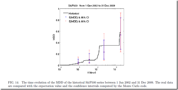
I think that the cumulative statistics, both total return and drawdown, fit well with the comment “The pictures imply that the maximum drawdown could have been pretty much anything.” Here is one of the figures that leads to this conclusion, and the predicted confidence interval from 20% to 90% is incredibly wide and not all that helpful.  If someone was willing to pay me for the bet that over the next 1,000 days, the S&P 500 or really any equity index drawdown falls between 20% and 90%, I would be happy to take that bet, and I would not need sophisticated statistical techniques to give me that insight.

image

Although I do not replicate the paper exactly with the most obvious difference that I use monthly returns 1950-May 2012 rather than daily returns 2002-2009, we can evaluate both return and drawdown through density plots with multiple distribution methods.  I limited my simulation to 10,000 samples so that I would not be up all night, but 10,000 is sufficient to show that over 62 years, both cumulative return and max drawdown can be virtually anything and both are “blazingly variable.”  I wonder how this would compare with life with sickness/death as drawdown and age of death as cumulative return.

From TimelyPortfolio

To be fair, let’s annualize the cumulative returns (actually probably better to do over 5 to 20 year periods).

From TimelyPortfolio

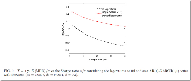
Independent of the outcome, I really enjoyed the paper’s Figures 8, 9, and 10 getting me one step closer to the question posed in my post Is Drawdown the Biggest Determinant of System Success?

image

image

image

We do see a relationship between return and drawdown.

From TimelyPortfolio

If nothing else, I was delighted to see a discussion of the often ignored drawdown statistic, which is the key to every investment decision I make.

R code from GIST:

Thursday, May 31, 2012

Conditional Drawdown Exploration

After reading Strub, Issam S., Trade Sizing Techniques for Drawdown and Tail Risk Control (May 21, 2012), I thought I should try to tie this with 2 other good R pieces on Conditional Drawdown:

http://systematicinvestor.wordpress.com/2011/11/01/minimizing-downside-risk/
http://www.rinfinance.com/agenda/2010/Carl+Peterson+Boudt_Tutorial.pdf

As always, NONE OF THIS IS INVESTMENT ADVICE.

In Strub’s paper, he uses conditional drawdown (CDaR) and conditional VaR (CVaR) to calculate the position size on directional (breakout determined) long/short currency positions.  The results were interesting enough to attempt to replicate with slight changes.  For this post, I will use CDaR to determine the position size on a long-only Mebane Faber 10-month moving average strategy.  We will start with an efficient frontier comparison and then abandon the frontier for a systematic approach.

(The blue text represents the added explanation in response to a comment)

If we look below at the frontier plots of return versus each measure of risk—the most common standard deviation, CDaR (conditional drawdown), and CVaR (conditional variance at risk)—we see that the frontiers are not noticeably different.  Visually, the most different and in a bad way, is the red CVaR line in the top left frontier plot.  The red CVaR line offers less return for each unit of standard deviation than the other two frontier lines, but the underperformance is not apparent when we use CDaR or CVaR on our x-axis as our measure of risk.

From TimelyPortfolio

Like the frontier plots above, the transition maps show only slightly different efficient allocations for each potential unit of risk.  At the lower end of the risk axis (left on the chart), we can see the biggest differences between allocations.

From TimelyPortfolio

The lack of noticeably different results seems consistent with well-known issues of mean-variance optimization.  These issues are described very well in this Morningstar piece.

“It is well known that mean-variance optimization is very sensitive to the estimates of returns, standard deviations, and correlations (see Michaud [1989] and Best and Grauer [1991]). Of these three inputs, returns are by far the most important and, unfortunately, the least stable. Chopra and Ziemba [1993] estimated that at a moderate risk tolerance level, mean-variance optimization is 11 times more sensitive to estimation error in returns relative to estimation error in risk (variance) and mean-variance optimization is two times more sensitive to estimation error in risk (variance) relative to estimation error in covariances (which also applies to correlations). Richard Michaud coined the phrase “the Markowitz optimization enigma” to describe the problem of input sensitivity and the highly concentrated asset allocations that result (see Michaud [1989]).

Input sensitivity indicates that the model’s output (the asset allocations) changes significantly due to small changes in the input (the capital market assumptions). Estimation error refers to the fact that in a forward-looking context the inputs are forecasts, and as such, are likely to be less than perfect (i.e. they contain errors). Putting these two issues together enables an uninformed practitioner to do more harm than good.”

For one more look at the lack of significant difference, let’s look at the cumulative returns of the 25th allocation from each efficient frontier.

From TimelyPortfolio

Even though the frontiers for the entire period are not significantly different, we can still use these more sophisticated risk measures in a different way to determine position size.  As a simple example similar to the example provided in Strub, let’s say we would like to pursue a Mebane Faber style 10-month moving average style long only position in each of the 3 currencies.  We would also like to limit the CDaR of each position to be 5%, so if we are fully allocated the sum of the 3 CDaR will be 15%. We will try to achieve this by using the 12 month rolling CDaR as our expected CDaR in the next month. Here is the chart of the 12 month rolling CDaR.

From TimelyPortfolio

If we just allocated 100% of the portfolio for each currency that exceeded its 10-month moving average, the results would look like this. Our maximum leverage across the portfolio would be 300%.

From TimelyPortfolio

However, if we would like to allocate more than 100% in quiet times and constrain our CDaR in volatile times, we can adjust our allocation by the 12 month rolling CDaR. As an example, if the New Zealand Dollar has a 15% CDaR for the last 12 months and we want 5% CDaR, we could allocate 33% or 15%historical/5%target to the New Zealand Dollar. This could result in a near infinite position size when CDaR is small, so we could also say that we want our maximum allocation to a single currency to be 200% or 600% at a portfolio level. The cumulative return chart would look like this.

From TimelyPortfolio

I think it very unlikely that this would be a final allocation mechanism, and I certainly would not be comfortable with this, but I hope it offers some instructive building blocks upon which you can build an allocation system.

R code from GIST:

Monday, April 23, 2012

Drawdown Look at Frontier of Assets and Systems

In Efficient Frontier of Funds and Allocation Systems, I had hoped to start exploring how a frontier can potentially be created with only one asset, or how an even more efficient frontier could be created with assets and also systems on those assets.  I am obsessed with drawdown, so of course I need to extend that post with a look at drawdown to satisfy this obsession. If you have not read the original post, please read it before this, since I will only show the additional graph created.

From TimelyPortfolio

R code from GIST:

Thursday, December 1, 2011

Is Drawdown the Biggest Determinant of System Success?

In all my system development, I still have not been able to determine what universal underlying conditions significantly improve a system’s chances of outperforming buy-and-hold.  Also, I have found very little discussion, so maybe R with some help from ttrTests can help answer my question of when I should just go buy-and-hold (a very pleasant situation for a money manager).  Starting in this business in 1998, I have often said that I dream of a day when I can just buy and hold similar to Japan stocks 1980-1990, US stocks 1990-2000, and US bonds 1982-now.

Those who follow my blog or know me already understand my obsession with drawdown, but that obsession focuses more on client/manager psychology (Investing for the Long Run) rather than drawdown’s effects on tactical systems.  I do not understand the industry’s focus on standard deviation.  I have never had a client call me or even worse fire me because my standard deviation has increased.  I know the argument is that higher standard deviations lead to higher drawdown, but as I show later in the post, this does not seem to be the case.

Clients call me or fire me because they have lost money, so if I can minimize the frequency, amplitude, and duration of drawdowns, then I can help/guide the client and reduce the worry, which is one main reason why they are paying me.  Also, though I think that focusing on minimizing drawdown can meaningfully increase the chances of achieving their long term return objectives (Drawdown Control Can Also Determine Ending Wealth and Confidence, Ending Equity, and What I Can Do as the Money Manager), which is even more likely the reason why clients pay me.

How nice would it be if drawdown also determines an objective system’s success?  To start the testing I thought I would use the fine work of David St. John on ttrTests (ttrTests 4th and Final Test) to get 100,000 bootstrapped samples from monthly S&P 500 data to examine drawdown, standard deviation, skewness, and compound returns on buy-and-hold versus a Mebane Faber 10-month moving average system.  Since I am so biased, I will let you determine the significance of drawdown on the results.

From TimelyPortfolio

Here is where I get some confidence in my belief higher standard deviation does not necessarily cause worse drawdowns. However, it is interesting that higher standard deviation has as high a correlation as drawdown with system out(under)performance (bottom right).

From TimelyPortfolio

R code from GIST:

Tuesday, August 23, 2011

Drawdown Visualization Supplement

As commented on Drawdown Visualization,

“Also, take a look at the example in ?chart.Event for another visualization of drawdowns, in this case stacking them for comparison.”

the PerformanceAnalytics package offers a very helpful look at the path of drawdowns that we can apply to financial and economic time series.  Here is the result applied to the Dow Jones Industrial Average since 1896.

From TimelyPortfolio

1929-1954 really messes this chart up, so let's limit the recovery to 750 days to get a better visualization.

From TimelyPortfolio

I thought it would be even more fun to apply this example to the GDP series.  This could be extended to all sorts of interesting economic data—first in my mind are industrial production and consumer spending.

From TimelyPortfolio


R code (click to download from Google Docs):

require(quantmod)
require(PerformanceAnalytics)   getSymbols("DJIA",src="FRED")
getSymbols("DJTA",src="FRED")
getSymbols("DJUA",src="FRED")   DJ <- merge(DJIA,DJTA,DJUA)   #DJ.yearly <- DJ[endpoints(DJ, on="years", k=1),]
DJ.roc <- ROC(DJ,n=1,type="discrete")     #another method of viewing drawdowns
#this is really easy with PerformanceAnalytics
#here is how to apply the very nice example
#provided in the documentation   DJ.draw = Drawdowns(DJ.roc[,1])
drawdowns = table.Drawdowns(DJ.roc[,1])
#jpeg(filename="DJIA worst drawdown event chart.jpg",
# quality=100,width=6.25, height = 6.25, units="in",res=96)
chart.Events(DJ.draw,
dates = drawdowns$Trough, prior=max(na.omit(drawdowns$"To Trough")),
post=max(na.omit(drawdowns$Recovery)),
lwd=2, colorset=redfocus, legend.loc=NULL,
main = "DJIA Worst Drawdowns")
#dev.off()
#drawdown is so long in 1929 that it messes up the chart
#let's limit this to two years or 750 trading days
#jpeg(filename="DJIA worst drawdown event chart with limit.jpg",
# quality=100,width=6.25, height = 6.25, units="in",res=96)
chart.Events(DJ.draw,
dates = drawdowns$Trough, prior=max(na.omit(drawdowns$"To Trough")),
post=min(750,max(na.omit(drawdowns$Recovery))),
lwd=2, colorset=redfocus, legend.loc=NULL,
main = "DJIA Worst Drawdowns
with Recovery Limit at 750 Days"
)
#dev.off()   #now let's do it for GDP
getSymbols("GDP",src="FRED")
GDP.roc <- ROC(GDP,type="discrete",n=1)
GDP.draw = Drawdowns(GDP.roc[,1])
drawdownsGDP = table.Drawdowns(GDP.roc[,1])
#jpeg(filename="GDP worst drawdown event chart.jpg",
# quality=100,width=6.25, height = 6.25, units="in",res=96)
chart.Events(GDP.draw,
dates = drawdownsGDP$Trough, prior=max(na.omit(drawdownsGDP$"To Trough")),
post=max(na.omit(drawdownsGDP$Recovery)),
lwd=2, colorset=redfocus, legend.loc="bottomright",xlab="Quarters +/- Drawdown",
main = "US GDP Worst Drawdowns")
#dev.off()

Created by Pretty R at inside-R.org

Monday, August 22, 2011

Drawdown Visualization

Drawdown is my favorite measure of risk.  It picks up extended autocorrelated pain often not seen in risk measures, and best illustrates frustration, panic, and loss of confidence (Drawdown Control Can Also Determine Ending Wealth).  I thought I should try some new ways to see it in R.  This first graph uses the zoo package to show 20% drawdowns in light pink and 40% drawdowns in darker pink.

From TimelyPortfolio

PerformanceAnalytics makes drawdown graphs and overlays very easy, but for some reason I got an error in findDrawdowns, so I instead used the table.Drawdowns function to see the 5 worst drawdowns.

From TimelyPortfolio

R code (click to download from Google Docs):

require(quantmod)
require(PerformanceAnalytics)   getSymbols("DJIA",src="FRED")
getSymbols("DJTA",src="FRED")
getSymbols("DJUA",src="FRED")   DJ <- merge(DJIA,DJTA,DJUA)   #DJ.yearly <- DJ[endpoints(DJ, on="years", k=1),]
DJ.roc <- ROC(DJ,n=1,type="discrete")
DJ.draw = Drawdowns(DJ.roc)   #jpeg(filename="DJ plot with Drawdowns zoo.jpg",
# quality=100,width=6.25, height = 6.25, units="in",res=96)
plot.zoo(log(DJ),plot.type="single",
col=c(2,3,4),ylab="log Price",xlab=NA,main="Dow Jones Indexes")
rgb <- hcl(c(0, 0, 260), c = c(100, 0, 100), l = c(50, 90, 50), alpha = 0.3)
xblocks(index(DJ),as.vector(DJ.draw[,1] < -0.20),col = rgb[1])
xblocks(index(DJ),as.vector(DJ.draw[,1] < -0.40),col = rgb[1])
legend("topleft",inset=0.05,colnames(DJ),fill=c(2,3,4),bg="white")
#dev.off()   #if we want to add linear models
#abline(lm(log(coredata(DJ[,1]))~as.Date(index(DJ))),col=2)
#abline(lm(log(coredata(DJ[,2]))~as.Date(index(DJ))),col=3)
#abline(lm(log(coredata(DJ[,3]))~as.Date(index(DJ))),col=4)     #another method of viewing drawdowns
#this is really easy with PerformanceAnalytics
#but for some reason I am getting an error
#with findDrawdowns
#will just shade worst drawdowns until I figure it out
drawdowns <- table.Drawdowns(DJ.roc[,1])
drawdowns.dates <- cbind(format(drawdowns$From),format(drawdowns$To))
drawdowns.dates[is.na(drawdowns.dates)] <- format(index(DJ.roc)[NROW(DJ.roc)])
# to get in proper list format
# thanks http://stackoverflow.com/questions/6819804/how-to-convert-a-matrix-to-a-list-in-r
drawdowns.dates <- lapply(seq_len(nrow(drawdowns.dates)), function(i) drawdowns.dates[i,])   #jpeg(filename="DJ plot with Drawdowns chart TimeSeries.jpg",
# quality=100,width=6.25, height = 6.25, units="in",res=96)
chart.TimeSeries(DJ,ylog=TRUE,
period.areas = drawdowns.dates,period.color = rgb[1],
colorset=c(2,3,4),
legend.loc="topleft",
main = "Dow Jones Indexes" )
#dev.off()
#or even fancier
#jpeg(filename="DJ plot with Drawdowns chart PerformanceSummary.jpg",
# quality=100,width=6.25, height = 8.25, units="in",res=96)
charts.PerformanceSummary(DJ.roc,ylog=TRUE,
period.areas = drawdowns.dates,period.color = rgb[1],
colorset=c(2,3,4),
legend.loc="topleft",
main = "Dow Jones Indexes" )
#dev.off()

Created by Pretty R at inside-R.org

Monday, July 11, 2011

Drawdown Control Can Also Determine Ending Wealth

As an extension to yesterday’s post Just Arriving is Not Enough, I wanted to show how minimizing drawdown is a much better technique to help control comfort and potentially increase ending wealth.  CHTTX was one of the best performers of the four funds OAKMX, CHTTX, FAIRX, and FCTNX mentioned in Smart Money “Bouncing Back with the World’s Greatest Investors.”  The fund suffered a brutal 60% drawdown though, and I’m guessing most of the original investors did not stick with the fund the entire time as the pain forced them out.  However, if we can limit the drawdown to something better than the excruciating 60%, then the ride is much smoother, or if someone truly is comfortable with 60% drawdown, we can apply leverage (I absolutely do not recommend) to both tailor the smoothness of our ride and also significantly increase ending wealth.

From TimelyPortfolio

We could apply up to 2.57 times leverage and incur the same drawdown as CHTTX, but let’s use a more conservative 2 times to see how it affects our simple system.

From TimelyPortfolio

In addition, if I as the money manager apply some drawdown control to my clients’ portfolio, I can help maintain their confidence and also significantly increase their ending wealth by not forcing them to make a decision based on fear.

R code (click to download):

#look at funds run by Smart Money's "world's greatest investors"
#http://www.smartmoney.com/invest/stocks/bouncing-back-with-the-worlds-greatest-investors-1309909342753/?cid=sm_dailyfinanceRSS
#then apply a simple moving average system
#to prove a point about controlling drawdown   require(quantmod)
require(PerformanceAnalytics)   tckr<-c("OAKMX","CHTTX","FAIRX","FCNTX")   start<-"1990-01-01"
end<- format(Sys.Date(),"%Y-%m-%d") # yyyy-mm-dd   # Pull tckr index data from Yahoo! Finance
getSymbols(tckr, from=start, to=end, adjust=TRUE)   RetToAnalyze<-merge(dailyReturn(OAKMX),dailyReturn(CHTTX),
dailyReturn(FAIRX), dailyReturn(FCNTX))
colnames(RetToAnalyze)<-tckr   #get very helpful Ken French data on Momentum Portfolios
#to compare to the funds
#http://mba.tuck.dartmouth.edu/pages/faculty/ken.french/ftp/6_Portfolios_ME_Prior_12_2_Daily.zip   my.url="http://mba.tuck.dartmouth.edu/pages/faculty/ken.french/ftp/6_Portfolios_ME_Prior_12_2_Daily.zip"
my.tempfile<-paste(tempdir(),"\\frenchmomentum.zip",sep="")
my.usefile<-paste(tempdir(),"\\6_Portfolios_ME_Prior_12_2_Daily.txt",sep="")
download.file(my.url, my.tempfile, method="auto",
quiet = FALSE, mode = "wb",cacheOK = TRUE)
unzip(my.tempfile,exdir=tempdir(),junkpath=TRUE)
#read space delimited text file extracted from zip
french_momentum <- read.table(file=my.usefile,
header = TRUE, sep = "",
as.is = TRUE,
skip = 12, nrows=12061)
colnames(french_momentum) <- c(paste("Small",
colnames(french_momentum)[1:3],sep="."),
paste("Large",colnames(french_momentum)[1:3],sep="."))   #get dates ready for xts index
datestoformat <- rownames(french_momentum)
datestoformat <- paste(substr(datestoformat,1,4),
substr(datestoformat,5,6),substr(datestoformat,7,8),sep="-")   #get xts for analysis
french_momentum_xts <- as.xts(french_momentum[,1:6],
order.by=as.Date(datestoformat))
#divide by 100 to get in decimal form
french_momentum_xts <- french_momentum_xts/100   #get column 3 for small momentum and 6 for large momentum
#to compare with the funds
RetWithFrench <-merge(RetToAnalyze,french_momentum_xts[,c(3,6)])   #jpeg(filename="performance summary of funds.jpg",quality=100,width=6.25, height = 8, units="in",res=96)
#charts.PerformanceSummary(RetWithFrench,ylog=TRUE,
# main="Smart Money World's Greatest Investors???",
# colorset=c("cadetblue","darkolivegreen3","goldenrod",
# "purple","gray","beige"))
#dev.off()   #let's just use a Mebane Faber style 200 day moving average
#to determine entry and exit
#for the best performer CHTTX
signal <- ifelse(CHTTX[,4]>runMean(CHTTX[,4],200),1,0)
signal <- merge(lag(signal,k=1),RetWithFrench[,2])
retCHTTX <- merge(signal[,1] * signal[,2], signal[,2])
colnames(retCHTTX) <- c("CHTTXMeanSystem","CHTTX")
#jpeg(filename="performance summary of chttx and mean system.jpg",quality=100,width=6.25, height = 8, units="in",res=96)
charts.PerformanceSummary(retCHTTX,ylog=TRUE,
main="Smart Money World's Greatest Investors???
CHTTX with 200 Day Mean System"
,
colorset=c("cadetblue","purple"))
#dev.off()   #if the investor is comfortable with 60% drawdown
#then they should be comfortable with leverage applied
#to the simple mean system; 2.57 would make them even
#in terms of max drawdown
#jpeg(filename="worst drawdown of chttx and mean system.jpg",quality=100,width=6.25, height = 8, units="in",res=96)
barplot(maxDrawdown(retCHTTX), main="Worst Drawdown Comparison",
ylim=c(0,0.6))
dev.off()
#print(maxDrawdown(retCHTTX[,2])/maxDrawdown(retCHTTX[,1]))   #let's see now what it looks like with just 2 times leverage
#applied to the simple mean system
retCHTTX <- merge(signal[,1] * signal[,2], signal[,1] * 2 * signal[,2], signal[,2])
colnames(retCHTTX) <- c("CHTTXMeanSystem","CHTTXMean2xLeverage","CHTTX")
#jpeg(filename="performance summary of chttx and mean system and leverage.jpg",quality=100,width=6.25, height = 8, units="in",res=96)
charts.PerformanceSummary(retCHTTX,ylog=TRUE,
main="Smart Money World's Greatest Investors???
CHTTX with 200 Day Mean System and 2x Leverage"
,
colorset=c("cadetblue","darkolivegreen3","purple"))
#dev.off()   #check max drawdown
#now by controlling drawdown we can end up with almost double the money
#with still less total drawdown
#jpeg(filename="worst drawdown of chttx and mean system with leverage.jpg",quality=100,width=6.25, height = 8, units="in",res=96)
barplot(maxDrawdown(retCHTTX), main="Worst Drawdown Comparison",
ylim=c(0,0.6))
#dev.off()
jpeg(filename="cumulative return of chttx and mean system with leverage.jpg",quality=100,width=6.25, height = 8, units="in",res=96)
barplot(Return.cumulative(retCHTTX), main="Cumulative Returns Comparison",
ylim=c(0,5))
dev.off()
print(Return.cumulative(retCHTTX[,2])/Return.cumulative(retCHTTX[,3]))

Created by Pretty R at inside-R.org

Sunday, July 10, 2011

Just Arriving is Not Enough

When you fly on an airplane, just arriving at your destination is not enough.  Almost all passengers want the ride to be super smooth and will sacrifice convenience and an on-time arrival to ensure comfort and perceived safety.  Also, passengers expect pilots to make this decision for them.  Like a pilot, I feel as a money manager, I bear the responsibility for the smoothness of my clients’ financial journey.  Unlike a pilot though, I have a much more significant burden since my clients can pull the emergency release as soon as they experience any discomfort.  Exiting due to panic or lack of confidence means my clients possibly make a financially fatal decision and either arrive late or never at their financial destination, so I must be even more cautious to not test the limits of my clients’ comfort.

When the ride is smooth, most of my clients do not care how fast I fly, but when the skies are unclear and the bumps severe, I need to take a different route (allocation) or not fly at all (sit in cash).  I would rather my client arrive a little late than to pull the emergency release and not arrive at all.  Pilots do not control the weather, and I do not control the markets, but we both must properly gauge conditions and make the decision to sacrifice convenience and an on-time arrival for a safe and comforable arrival.

Smart Money “Bouncing Back with the World’s Greatest Investors” does not seem to agree with my money management philosophy.  On the first manager Bill Nygren I see “Oakmark's 4 percent loss in 2007, and to a more dismal drop of 36 percent in 2008,” and these devastating drawdowns persist through the all four managers.  What troubles me most is how quickly the press and investors forgive pitiful performance and awful drawdowns in the crisis. These investors neither foresaw nor controlled the almost $10 trillion in political and monetary decisions required to temporarily rescue them. Here is a look at the mentioned funds.  Most of these managers simply avoided tech stocks in 2000-2003, but did nothing to avoid the far more severe disaster of 2007-2009.

From TimelyPortfolio

This is unacceptable to me, and I believe the flawed forgiveness will be punished in the next cycle as these managers, their investors, and the press learned nothing from the last crisis.

R code (click to download):

#look at funds run by Smart Money's "world's greatest investors"
#http://www.smartmoney.com/invest/stocks/bouncing-back-with-the-worlds-greatest-investors-1309909342753/?cid=sm_dailyfinanceRSS   require(quantmod)
require(PerformanceAnalytics)   tckr<-c("OAKMX","CHTTX","FAIRX","FCNTX")   start<-"1990-01-01"
end<- format(Sys.Date(),"%Y-%m-%d") # yyyy-mm-dd   # Pull tckr index data from Yahoo! Finance
getSymbols(tckr, from=start, to=end, adjust=TRUE)   RetToAnalyze<-merge(dailyReturn(OAKMX),dailyReturn(CHTTX),
dailyReturn(FAIRX), dailyReturn(FCNTX))
colnames(RetToAnalyze)<-tckr   #get very helpful Ken French data on Momentum Portfolios
#to compare to the funds
#http://mba.tuck.dartmouth.edu/pages/faculty/ken.french/ftp/6_Portfolios_ME_Prior_12_2_Daily.zip   my.url="http://mba.tuck.dartmouth.edu/pages/faculty/ken.french/ftp/6_Portfolios_ME_Prior_12_2_Daily.zip"
my.tempfile<-paste(tempdir(),"\\frenchmomentum.zip",sep="")
my.usefile<-paste(tempdir(),"\\6_Portfolios_ME_Prior_12_2_Daily.txt",sep="")
download.file(my.url, my.tempfile, method="auto",
quiet = FALSE, mode = "wb",cacheOK = TRUE)
unzip(my.tempfile,exdir=tempdir(),junkpath=TRUE)
#read space delimited text file extracted from zip
french_momentum <- read.table(file=my.usefile,
header = TRUE, sep = "",
as.is = TRUE,
skip = 12, nrows=12061)
colnames(french_momentum) <- c(paste("Small",
colnames(french_momentum)[1:3],sep="."),
paste("Large",colnames(french_momentum)[1:3],sep="."))   #get dates ready for xts index
datestoformat <- rownames(french_momentum)
datestoformat <- paste(substr(datestoformat,1,4),
substr(datestoformat,5,6),substr(datestoformat,7,8),sep="-")   #get xts for analysis
french_momentum_xts <- as.xts(french_momentum[,1:6],
order.by=as.Date(datestoformat))
#divide by 100 to get in decimal form
french_momentum_xts <- french_momentum_xts/100   #get column 3 for small momentum and 6 for large momentum
#to compare with the funds
RetWithFrench <-merge(RetToAnalyze,french_momentum_xts[,c(3,6)])     jpeg(filename="performance summary of funds.jpg",quality=100,width=6.25, height = 8, units="in",res=96)
charts.PerformanceSummary(RetWithFrench["2003-03::2011-05",],ylog=TRUE,
main="Smart Money World's Greatest Investors???",
colorset=c("cadetblue","darkolivegreen3","goldenrod",
"purple","gray","beige"))
dev.off()

Created by Pretty R at inside-R.org