Showing posts with label cfa. Show all posts

Thursday, January 10, 2013

Interesting Presentation from Van Eck Trackers Team

I just saw a very interesting presentation from the Van Eck Trackers Team (acquired by Van Eck in July 2012) at the CFA Society of Alabama January 2013 lunch.  I have not had the chance to read all their research and attempt to replicate portions in R, but I found two points very compelling.  First, the research done on the price of illiquidity

Freed, Marc S., and Ben McMillan. "Investible Benchmarks and Hedge Fund Liquidity." The Journal of Wealth Management 14.3: 58-66.

published in the Journal of Wealth Management potentially could inversely answer the pricing of Warren Buffett’s notion of “cash as a call option” described in a Globe and Mail article with my own thoughts in this post.  The price of illiquidity can be considerable as shown below,

image

so inversely the opportunity from liquidity or available cash could be substantial. Imagine what hedge fund performance might look like net of fee, net of tax, and net of illiquidity. Even the best managers cannot achieve a high enough return to compensate for this level of embedded costs.  Strangely enough it also comes close to my crude heuristic of 10% expected return premium necessary for me to justify illiquidity.

The presentation (similar presentation given to the CFA Society of Pittsburgh) also discusses the concept of True® Alpha.  The decomposition is nicely described in this graphic from the presentation.

image 

I have not confirmed with the authors/speakers their use of R, but their were some remarkably familiar graph layouts that lead me to believe R played a prominent role.  Regardless, I would really like to replicate some of the calculations in R.

Wednesday, February 1, 2012

Jim Rogers at CFA Society of Alabama Dinner

I am extremely excited to share the announcement that Jim Rogers will present at the CFA Society of Alabama Annual Dinner February 29 at Barber Motorsports Museum in Birmingham.  I believe there is still room for anyone who might like to attend.  Barron’s senior editor Jack Willoughby will moderate.  Congratulations to the CFA Society of Alabama on a high-powered event.

image

Friday, June 24, 2011

Confidence, Ending Equity, and What I Can Do as the Money Manager

I wrote this as my quarterly commentary, but I thought I should share it as a general discussion piece.  More than on any post, I would absolutely love feedback and comments good or bad.

Confidence, Money Management, and Your Wealth

How would you respond if this were your money manager (revealed later) in 1974? Would you have added or subtracted money? Although I do not know your answer, I probably would have subtracted money or closed the account entirely.

image

Data Provided by Statman, Meir and Scheid, Jonathan, Buffett in Foresight and Hindsight (September 2001). Santa Clara University Working Paper No. 00/01-37.Available at SSRN: http://ssrn.com/abstract=277161

Your ending wealth depends much more on when and how much money you add or subtract than how well I perform. While I can manage risk and return as your money manager, I unfortunately cannot control this most important determinant of your ending wealth. Without confidence, money management fails, so what I do to build and maintain your confidence probably will build your wealth more than my geometrically linked returns. My method for building and maintaining your confidence and ultimately your ending wealth requires two elements: open honest communication and drawdown minimization.

1) Open honest communication requires your help, since the conversation needs to go both ways. I will continue to send quarterly updates and performance reports, but I also need to know your feelings, concerns, suggestions, questions, life changes, or really anything so I can help achieve your financial objectives. I am available by phone, email, mail, face-to-face, text message, Twitter, Skype, and IM.

2) In the chart above, my guess is your decision was based more on the money lost than the underperformance. Fear crushes confidence, and if I can keep drawdowns under 10-15%, then both the duration and magnitude of your fear will be greatly relieved.

How would you feel if you dumped Berkshire Hathaway and Warren Buffett in 1976? The manager in the above chart was Warren Buffett, and if you retained Buffett/Berkshire through 2010, you would have made $161 million more on an initial $100,000 investment than the S&P 500. I in no way claim an ability to replicate Warren Buffett’s performance or management style, but I think this offers a good illustration of how even one of the world’s all-time best money managers could have lost his clients’ confidence and potentially impacted their ending net worth.

In Forbes Oct 29, 1998 The Berkshire Bunch, Buffett says "The first investors just believed in me. The ones who had faith stayed on; you couldn't get my Aunt Katie to sell if you came at her with a crowbar. But the people who came in later because they thought the stock was cheap and they were attracted to my record didn't always stay. It's a process of natural selection."


As I said, I would love to hear your thoughts. I limited the piece to one page, but another very good related piece can be found at

Opportunities for Patient Investors, Jason Zwieg and Seth Klarman

Financial Analysts Journal, September/October 2010, Vol. 66, No. 5:18-28.

I did the chart in Excel, but I thought I would include the Buffett dataset (click for the file) in R also.  Here is what it looks like.

From TimelyPortfolio

R code (click to download):

require(quantmod)
require(PerformanceAnalytics)
require(ggplot2)   berkshire_sp500 <- read.csv("berkshire_and_sp500.csv",stringsAsFactors=FALSE)
berkshire_sp500 <- as.xts(berkshire_sp500[,2:3],order.by=as.Date(berkshire_sp500[,1]))   #annual data unfortunately does not work with PerformanceAnalytics
#so these won't look as good as I would like   #calculate growth of $1
#first step is getting returns
cumPerf <- ROC(berkshire_sp500,n=1,type="discrete")
#remove na from start of series
cumPerf[1,] <- 0
#second step is calculating the cumulative product of returns
#or geometrically link the periodic returns
cumPerf[,1] <- cumprod(1+cumPerf[,1])
cumPerf[,2] <- cumprod(1+(cumPerf[,2]))   #get df from the xts
df <- data.frame(cbind(index(cumPerf),data.matrix(coredata(cumPerf[,1:2]))))
#name columns
colnames(df) <- c("Date",colnames(df)[2:3])
#use melt to get in format that ggplot likes best
df <- melt(df,id=1)
colnames(df) <- c("Date","Investment","GrowthOfDollar")
#jpeg(filename="GrowthOfDollar.jpg",quality=100,width=6.25, height = 5, 
# units="in",res=96)
ggplot(df,aes(x=Date,y=GrowthOfDollar,colour=Investment)) +
geom_line() + scale_x_date(major="5 years",format="%Y") +
scale_y_log10() + opts(title = "Berkshire and S&P 500 Growth of $1 
1965-2010")
#dev.off()

Created by Pretty R at inside-R.org

Tuesday, May 24, 2011

Utility Spread and Financial Turbulence Part 2 with Utility Slope

THIS IS NOT INVESTMENT ADVICE.  YOU ARE RESPONSIBLE FOR YOUR OWN GAINS AND LOSSES.

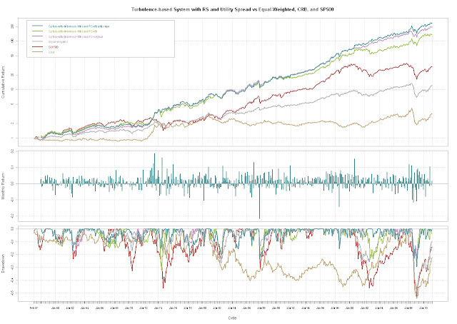
I did not intend for this to be a two-part series but I just could not be complacent with Utility Spread and Financial Turbulence (for avid readers, there was a small error in this post that is now corrected).  Since the change was so easy and the results so much better, I thought I should share.

In previous posts, I set up a very basic relative strength approach by using the 12 month slope (linear beta) to choose the stronger performer.  The improvements from adding this relative strength technique to my original Great FAJ Article on Statistical Measure of Financial Turbulence system were substantial as seen in Great FAJ Article on Statistical Measure of Financial Turbulence Part 3.  If the technique has helped in the past and I already know how to do the calculation, I figured I should at least try to apply it to the Utility Spread.  Now when turbulence is low, invest in the stronger of the S&P 500 and CRB, but when turbulence is high, use the Utility Spread only if its 12 month slope is positive.  If everything is blowing up (turbulence high) and utilities are not defensive (slope is negative), then use the US 10y Treasury as your last resort.  Lots of rules but they intuitively make sense to me.  Drawdown remains higher than I would like.

From TimelyPortfolio

R code (thanks patrick for the comment to make code more readable):

#cleaned up the code to eliminate leftovers from previous posts and studies
#see http://timelyportfolio.blogspot.com for the history and older code   require(quantmod)
require(PerformanceAnalytics)   #get data from St. Louis Federal Reserve (FRED)
getSymbols("GS20",src="FRED") #load 20yTreasury; 20y has gap 86-93; 30y has gap in early 2000s
getSymbols("GS30",src="FRED") #load 30yTreasury to fill 20y gap 86-93
getSymbols("GS10",src="FRED") #load 10yTreasury
getSymbols("BAA",src="FRED") #load BAA
getSymbols("SP500",src="FRED") #load SP500
#now Dow Jones Indexes
getSymbols("DJIA",src="FRED") #load daily Dow Jones Industrial
getSymbols("DJUA",src="FRED") #load daily Dow Jones Utility   DJUADJIA <- DJUA/DJIA   #get CRB data from a csv file
CRB <- as.xts(read.csv("crb.csv",row.names=1))[,1]   #fill 20y gap from discontinued 20y Treasuries with 30y
GS20["1987-01::1993-09"] <- GS30["1987-01::1993-09"]   #do a little manipulation to get the data lined up on monthly basis
SP500 <- to.monthly(SP500)[,4]
GS10 <- to.monthly(GS10)[,4]
DJUADJIA <- to.monthly(DJUADJIA)[,4]
#get monthly format to yyyy-mm-dd with the first day of the month
index(SP500) <- as.Date(index(SP500))
index(GS10) <- as.Date(index(GS10))
index(DJUADJIA) <- as.Date(index(DJUADJIA))
#my CRB data is end of month; could change but more fun to do in R
CRB <- to.monthly(CRB)[,4]
index(CRB) <- as.Date(index(CRB))   #let's merge all this into one xts object; CRB starts last in 1956
assets <- na.omit(merge(GS20,SP500,CRB,DJUADJIA))
#use ROC for SP500 and CRB and momentum for yield data
assetROC <- na.omit(merge(momentum(assets[,1])/100,ROC(assets[,2:4],type="discrete")))   ############Turbulence calculation
#get Correlations
corrBondsSp <- runCor(assetROC[,1],assetROC[,2],n=7)
corrBondsCrb <- runCor(assetROC[,1],assetROC[,3],n=7)
corrSpCrb <- runCor(assetROC[,2],assetROC[,3],n=7)
#composite measure of correlations between asset classes and roc-weighted correlations
assetCorr <- (corrBondsSp+corrBondsCrb+corrSpCrb+
(corrBondsSp*corrSpCrb*assetROC[,2])+
(corrBondsCrb*corrSpCrb*assetROC[,3])-
assetROC[,1])/6
#sum of ROCs of asset classes
assetROCSum <- assetROC[,1]+assetROC[,2]+assetROC[,3]
#finally the turbulence measure
turbulence <- abs(assetCorr*assetROCSum*100)
colnames(turbulence) <- "Turbulence-correlation"
############   ############Get Bond Return Data
#get bond returns to avoid proprietary data problems
#see previous timelyportfolio blogposts for explanation
#probably need to make this a function since I will be using so much
require(RQuantLib)
GS10pricereturn <- GS10 #set this up to hold price returns   GS10pricereturn[1,1] <- 0
colnames(GS10pricereturn) <- "BondPriceReturn"
#I know I need to vectorize this but not qualified enough yet
#Please feel free to comment to show me how to do this
for (i in 1:(NROW(GS10)-1)) {
GS10pricereturn[i+1,1] <- FixedRateBondPriceByYield(yield=GS10[i+1,1]/100,issueDate=Sys.Date(),
maturityDate= advance("UnitedStates/GovernmentBond", Sys.Date(), 10, 3),
rates=GS10[i,1]/100,period=2)[1]/100-1
}   #interest return will be yield/12 for one month
GS10interestreturn <- lag(GS10,k=1)/12/100
colnames(GS10interestreturn) <- "BondInterestReturn"   #total return will be the price return + interest return
GS10totalreturn <- GS10pricereturn + GS10interestreturn
colnames(GS10totalreturn) <- "BondTotalReturn"
assetROC <- na.omit(merge(GS10totalreturn,ROC(assets[,2:4],type="discrete")))
############   ############System building
#wish I could remember where I got some of this code
#most likely candidate is www.fosstrading.com
#please let me know if you know the source
#so I can give adequate credit   #let's use basic relative strength to pick sp500 or crb
#know I can do this better in R but here is my ugly code
#to calculate 12 month slope of sp500/crb and djua/djia
width=12
for (i in 1:(NROW(assets)-width)) {
#get sp500/crb slope
model <- lm(assets[i:(i+width),2]/assets[i:(i+width),3]~index(assets[i:(i+width)]))
ifelse(i==1,assetSlope <- model$coefficients[2],assetSlope <- rbind(assetSlope,model$coefficients[2]))
#get djua/djia slope; already calculated ratio so just take that
model_util <- lm(assets[i:(i+width),4]~index(assets[i:(i+width)]))
ifelse(i==1,assetSlopeUtil <- model_util$coefficients[2],assetSlopeUtil <- rbind(assetSlopeUtil,model_util$coefficients[2]))
}
assetSlope <- xts(cbind(assetSlope),order.by=index(assets)[(width+1):NROW(assets)])
assetSlopeUtil <- xts(cbind(assetSlopeUtil),order.by=index(assets)[(width+1):NROW(assets)])
assetSlope <- merge(assetSlope,assetSlopeUtil)
#use turbulence to determine in or out of equal-weighted sp500 and crb
signal <- ifelse(turbulence>0.8,0,1)   #use slope of sp500/crb to determine sp500 or crb
signal2 <- ifelse(assetSlope[,1]>0,1,2)   #lag signals
#if we knew what would happen tomorrow, we can eliminate all this effort
signal <- lag(signal,k=1)
signal[1] <- 0
signal2 <- lag(signal2,k=1)
signal2[1] <- 0   signals_returns <- merge(signal,signal2,assetROC,assetSlope)
#get sp500 or crb return based on slope when turbulence low or use bonds as cash
ret <- ifelse(signals_returns[,2]==1&signals_returns[,1]==1,signals_returns[,4],
ifelse(signals_returns[,2]==2&signals_returns[,1]==1,signals_returns[,5],
signals_returns[,3]))
#get sp500 or crb return based on slope when turbulence low or use utility spread as cash
ret_util <- ifelse(signals_returns[,2]==1&signals_returns[,1]==1,signals_returns[,4],
ifelse(signals_returns[,2]==2&signals_returns[,1]==1,signals_returns[,5],
signals_returns[,6]))
#get sp500 or crb return based on slope when turbulence low or use utility spread
#as cash only if slope positive
ret_util_slope <- ifelse(signals_returns[,2]==1&signals_returns[,1]==1,signals_returns[,4],
ifelse(signals_returns[,2]==2&signals_returns[,1]==1,signals_returns[,5],
ifelse(signals_returns[,8]>0,signals_returns[,6],signals_returns[,3])))
ret_util[1] <- 0
ret_util_slope[1] <- 0   #get system performance
system_perf_rs <- ret
system_perf_rs_util <- ret_util
system_perf_rs_util_slope <- ret_util_slope   perf_comparison <- merge(system_perf_rs_util_slope,system_perf_rs_util,system_perf_rs,(assetROC[,2]+assetROC[,3])/2,assetROC[,2],assetROC[,3])
colnames(perf_comparison) <- c("System-with-turbulence-filter and RS-util with slope",
"System-with-turbulence-filter and RS-util", "System-with-turbulence-filter and RS-original",
"Equal-weighted","S&P500","CRB")   charts.PerformanceSummary(perf_comparison,ylog=TRUE,
main="Turbulence-based System with RS and Utility Spread vs Equal-Weighted, CRB, and SP500",
colorset=c("cadetblue","darkolivegreen3","plum3","gray70","indianred","burlywood3"))

Created by Pretty R at inside-R.org

Monday, May 23, 2011

Utility Spread and Financial Turbulence

THIS IS NOT INVESTMENT ADVICE.  YOU ARE RESPONSIBLE FOR YOUR OWN GAINS AND LOSSES.

In Long XLU Short SPY Part 2 (More History), I explored the defensive nature of the spread and its potential as a bond substitute in troublesome periods for stocks.  I thought it would be interesting to see what happens if we use the spread as our cash position in the Great FAJ Article on Statistical Measure of Financial Turbulence Part 3 system.  Unfortunately, the use of the spread on price returns as cash does not benefit the system as much as bonds as cash, but I still thought it might encourage some additional reader thought on the spread and its potential uses.

From TimelyPortfolio

R code:

require(quantmod)
require(PerformanceAnalytics)

#get data from St. Louis Federal Reserve (FRED)
getSymbols("GS20",src="FRED") #load 20yTreasury; 20y has gap 86-93; 30y has gap in early 2000s
getSymbols("GS30",src="FRED") #load 30yTreasury to fill 20y gap 86-93
getSymbols("BAA",src="FRED") #load BAA
getSymbols("SP500",src="FRED") #load SP500
#now Dow Jones Indexes
getSymbols("DJIA",src="FRED") #load daily Dow Jones Industrial
getSymbols("DJUA",src="FRED") #load daily Dow Jones Utility

DJUADJIA<-DJUA/DJIA

#get CRB data from a csv file
CRB<-as.xts(read.csv("crb.csv",row.names=1))[,1]

#fill 20y gap from discontinued 20y Treasuries with 30y
GS20["1987-01::1993-09"]<-GS30["1987-01::1993-09"]

#do a little manipulation to get the data lined up on monthly basis
SP500<-to.monthly(SP500)[,4]
DJUADJIA<-to.monthly(DJUADJIA)[,4]
#get monthly format to yyyy-mm-dd with the first day of the month
index(SP500)<-as.Date(index(SP500))
index(DJUADJIA)<-as.Date(index(DJUADJIA))
#my CRB data is end of month; could change but more fun to do in R
CRB<-to.monthly(CRB)[,4]
index(CRB)<-as.Date(index(CRB))

#let's merge all this into one xts object; CRB starts last in 1956
assets<-na.omit(merge(GS20,SP500,CRB,DJUADJIA))
#use ROC for SP500 and CRB and momentum for yield data
assetROC<-na.omit(merge(momentum(assets[,1])/100,ROC(assets[,2:4],type="discrete")))

#get Correlations
corrBondsSp<-runCor(assetROC[,1],assetROC[,2],n=7)
corrBondsCrb<-runCor(assetROC[,1],assetROC[,3],n=7)
corrSpCrb<-runCor(assetROC[,2],assetROC[,3],n=7)
#composite measure of correlations between asset classes and roc-weighted correlations
assetCorr<-(corrBondsSp+corrBondsCrb+corrSpCrb+
    (corrBondsSp*corrSpCrb*assetROC[,2])+
    (corrBondsCrb*corrSpCrb*assetROC[,3])-
    assetROC[,1])/6
#sum of ROCs of asset classes
assetROCSum<-assetROC[,1]+assetROC[,2]+assetROC[,3]
#finally the turbulence measure
turbulence<-abs(assetCorr*assetROCSum*100)
colnames(turbulence)<-"Turbulence-correlation"

chartSeries(turbulence,theme="white",name="Correlation and % Change as Measure of Financial Turbulence")
abline(h=0.8)

chart.ACF(turbulence,main="Auto-correlation of Turbulence")

#wish I could remember where I got some of this code
#most likely candidate is www.fosstrading.com
#please let me know if you know the source
#so I can give adequate credit

#use turbulence to determine in or out of equal-weighted sp500 and crb
signal<-ifelse(turbulence>0.8,0,1)
#use slope of sp500/crb to determine sp500 or crb

signal<-lag(signal,k=1)
# Replace missing signals with no position
# (generally just at beginning of series)
signal[is.na(signal)] <- 0

#get returns from equal-weighted crb and sp500 position; Return.portfolio was causing problems, so did the hard way
ret<-ifelse(signal==1,(assetROC[,2]+assetROC[,3])/2,assetROC[,4])
ret[1] <- 0

#get system performance
system_perf <- ret*signal
system_perf_util <- ret
system_eq <- cumprod(1+signal*ret)
system_eq_util <- cumprod(1+ret)

perf_comparison<-merge(lag((assetROC[,2]+assetROC[,3])/2,k=1),system_perf,system_perf_util)
colnames(perf_comparison)<-c("Equal-weighted","System-with-turbulence-filter","System-with-turbulence-filter-with-util")

charts.PerformanceSummary(perf_comparison,ylog=TRUE,main="Turbulence-based System vs Equal-Weighted CRB and SP500")

#let's use basic relative strength to pick sp500 or crb
#know I can do this better in R but here is my ugly code
#to calculate 12 month slope of sp500/crb
width=12
for (i in 1:(NROW(assets)-width)) {
    model<-lm(assets[i:(i+width),2]/assets[i:(i+width),3]~index(assets[i:(i+width)]))
    ifelse(i==1,assetSlope<-model$coefficients[2],assetSlope<-rbind(assetSlope,model$coefficients[2]))
}
assetSlope<-xts(cbind(assetSlope),order.by=index(assets)[(width+1):NROW(assets)])
#use turbulence to determine in or out of equal-weighted sp500 and crb
signal<-ifelse(turbulence>0.8,0,1)

#use slope of sp500/crb to determine sp500 or crb
signal2<-ifelse(assetSlope[,1]>0,1,2)

signal<-lag(signal,k=1)
signal[1]<-0
signal2<-lag(signal2,k=1)
signal2[1]<-0

signals_and_returns<-merge(signal,signal2,assetROC,assetSlope,turbulence)
#get sp500 or crb return based on slope when turbulence low or use bonds as cash
ret<-ifelse(signals_and_returns[,2]==1,signals_and_returns[,4],ifelse(signals_and_returns[,2]==2,signals_and_returns[,5],signals_and_returns[,3]))
#get sp500 or crb return based on slope when turbulence low or use utility spread as cash
ret_util<-ifelse(signals_and_returns[,2]==1&signals_and_returns[,1]==1,signals_and_returns[,4],
    ifelse(signals_and_returns[,2]==2&signals_and_returns[,1]==1,signals_and_returns[,5],
    signals_and_returns[,6]))
ret[1]<-0
ret_util[1]<-0

#get system performance
system_perf_rs<-signals_and_returns[,1]*ret
system_perf_rs_util<-ret_util
system_eq_rs<- cumprod(1+signals_and_returns[,1]*ret)
system_eq_rs_util<- cumprod(1+ret_util)

perf_comparison<-merge((assetROC[,2]+assetROC[,3])/2,assetROC[,2],assetROC[,3],system_perf,system_perf_util,system_perf_rs,system_perf_rs_util)
colnames(perf_comparison)<-c("Equal-weighted","S&P500","CRB","System-with-turbulence-filter","System-with-turbulence-filter-util","System-with-turbulence-filter and RS","System-with-turbulence-filter and RS-util")

charts.PerformanceSummary(perf_comparison,ylog=TRUE,main="Turbulence-based System with RS vs Equal-Weighted, CRB, and SP500")

Tuesday, May 17, 2011

Russell Napier, ASIP in FT Says Emerging Market Currencies

Clearly I have succumbed to confirmation bias, since my second favorite presentation from the CFA Institute Annual Conference this year came from Scotland native Russell Napier, ASIP who shares my views nearly completely http://video.ft.com/v/946244201001/Long-View-Historian-sees-S-P-fall-to-400.

From TimelyPortfolio

As one of the most bearish money managers in Barron’s Spring Big Money Poll, I get some strange looks with my forecast for S&P 500 at 900, so I cannot imagine how much resistance he gets with his S&P 500 potential price of 400.  However, given inappropriate responses to the next crisis or Napier’s “the great reset”, 900 to 400 is not entirely inconceivable.

“Kenton Russell, of the brokerage Sterne Agee, used to be bullish, but now makes no bones about being a bear. "The primary assumption people are making is dollar stability," he says. "If you don't pay attention to the dollar while being long bonds and stocks in the U.S., you are not paying attention to the most crucial element of the trade."

Based on the declining value of the dollar, which hit a 15-month low Wednesday against the euro, the market is "right back at the lows" seen before the financial crisis, Russell says. He expects stocks to drop about 20% in the next year or so, with investors selling the DJIA down to 9500 and the S&P to 900 as they come to realize the U.S. has "reached the limits of fiscal and monetary policy."

A 20% correction "is no collapse," Russell says, although some might argue it will feel like one. He recommends shorting the iShares Russell 2000 exchange-traded fund (IWM) and buying the iShares MSCI Emerging Markets ETF (EEM), as he thinks Asian currencies are undervalued.”

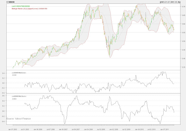
We both agree most strongly on our view on emerging market currencies.  In an attempt to link what I heard and learned last week at the conference with my blog and R, I thought I should update my March 2011 post Long EEM Short IWM-How it Works in 3 Ways.  The idea is easily analyzed in R and very easily pursued even by a retail investor.  For all the details please see the original post.  Here are the updated charts and a couple of new charts.

From TimelyPortfolio

R code:

require(quantmod)
require(PerformanceAnalytics)
require(fAssets)
require(ggplot2)

tckr<-c("EEM","IEF","IWM","GLD","SPY")

start<-"2005-01-01"
end<- format(Sys.Date(),"%Y-%m-%d") # yyyy-mm-dd

# Pull tckr index data from Yahoo! Finance
getSymbols(tckr, from=start, to=end)

EEM<-adjustOHLC(EEM,use.Adjusted=T)
IEF<-adjustOHLC(IEF,use.Adjusted=T)
IWM<-adjustOHLC(IWM,use.Adjusted=T)
GLD<-adjustOHLC(GLD,use.Adjusted=T)
SPY<-adjustOHLC(SPY,use.Adjusted=T)

EEM<-to.weekly(EEM, indexAt='endof')
IEF<-to.weekly(IEF, indexAt='endof')
IWM<-to.weekly(IWM, indexAt='endof')
GLD<-to.weekly(GLD, indexAt='endof')
SPY<-to.weekly(SPY, indexAt='endof')
EEMIWM<-to.weekly(EEM/IWM, indexAt='endof')

RetToAnalyze<-merge(weeklyReturn(EEM),weeklyReturn(IEF),weeklyReturn(IWM),weeklyReturn(GLD),weeklyReturn(SPY),weeklyReturn(EEMIWM))
colnames(RetToAnalyze)<-c(tckr,"EEMIWM")

assetsDendrogramPlot(as.timeSeries(RetToAnalyze))
assetsCorEigenPlot(as.timeSeries(RetToAnalyze))
mtext("Source: Yahoo! Finance",side=1,adj=0)

chart.Correlation(RetToAnalyze[,1:6,drop=F], main="Correlation since 2005")
mtext("Source: Yahoo! Finance",side=1,adj=0)

#get Rolling Correlations with IEF(bonds) and SPY(stocks)
corEEMIWMtoBonds<-runCor(RetToAnalyze[,6],RetToAnalyze[,2],25)
corEEMIWMtoStocks<-runCor(RetToAnalyze[,6],RetToAnalyze[,5],25)
chartSeries(EEMIWM,TA="addBBands();addTA(corEEMIWMtoBonds);addTA(corEEMIWMtoStocks)",theme="white")
mtext("Source: Yahoo! Finance",side=1,adj=0)

#downside risk comparison
downsideTable<-melt(cbind(rownames(table.DownsideRisk(RetToAnalyze)),table.DownsideRisk(RetToAnalyze)))
colnames(downsideTable)<-c("Statistic","Portfolio","Value")
ggplot(downsideTable, stat="identity", aes(x=Statistic,y=Value,fill=Portfolio)) + geom_bar(position="dodge") + coord_flip()
mtext("Source: Yahoo! Finance",side=1,adj=0)

chart.Boxplot(RetToAnalyze,main="Box Plot of Various Assets 2005 to May 2011")
mtext("Source: Yahoo! Finance",side=1,adj=0)

assetsRiskReturnPlot(RetToAnalyze)

table.CaptureRatios(RetToAnalyze[,6],RetToAnalyze[,5])
pfolioHist(RetToAnalyze[,6])
assetsMomentsPlot(as.timeSeries(RetToAnalyze), main="Plot of Moments of Various Assets since 2005")

Monday, May 16, 2011

Omega as Optimizer

During Jan Straatman’s presentation, I tweeted

Jan Straatman #cfa2011 In real life no normal distributions so use omega function to optimize actual returns

After the presentation, I asked Jan his second choice for optimization after Omega, and he responded nothing.  He added that he greatly dislikes optimization and avoids any optimization unless it is absolutely necessary.   Even though I share his dislike for optimization and avoid its temptations, I thought playing with Omega in R might offer a nice example of this very useful function.

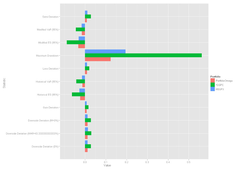
A very basic use of Omega might allow a Relative Strength style strategy for building an equity portfolio.  For those unfamiliar with the Hussman Strategic Growth Fund (HSGFX), it offers an absolute return style equity strategy (see blog posts his own drummer and The Timing Value of John Hussman’s Market Climate Assessments).  Feel free to play with other funds or indicies, but I thought we could build a nice basic portfolio with HSGFX and the S&P 500 just by investing in the investment with the higher Omega as long as the Omega exceeds 1.5.

The portfolio looks like this.

From TimelyPortfolio

Some working papers on SSRN regarding Omega are

http://papers.ssrn.com/sol3/papers.cfm?abstract_id=365740

http://papers.ssrn.com/sol3/papers.cfm?abstract_id=1289269

http://papers.ssrn.com/sol3/papers.cfm?abstract_id=910233

http://papers.ssrn.com/sol3/papers.cfm?abstract_id=557128&rec=1&srcabs=365740

Jan no longer posts his work on SSRN, but here are some of his older working papers http://papers.ssrn.com/sol3/cf_dev/AbsByAuth.cfm?per_id=485183.  Also, here is a nice article from the Financial Times.

R code:

require(quantmod)
require(PerformanceAnalytics)
require(ggplot2)

tckr<-c("^GSPC","HSGFX")

#define start and end dates
#Hussman starts 2000 but I use 1990 in case you want to look at other funds
start<-"1990-12-31"
end<- format(Sys.Date(),"%Y-%m-%d") # yyyy-mm-dd

# Pull adjusted tckr index data from Yahoo! Finance
getSymbols(tckr, from=start, to=end, adjust=TRUE)

# move from daily to weekly
GSPC<-to.weekly(GSPC, indexAt='endof')[,4]
HSGFX<-to.weekly(HSGFX, indexAt='endof')[,4]

# convert price data to return data for analysis with PerformanceAnalytics
GSPC<-weeklyReturn(GSPC)
HSGFX<-weeklyReturn(HSGFX)

# merge the two series
RetToAnalyze<-na.omit(merge(GSPC,HSGFX))
colnames(RetToAnalyze)<-tckr

#some charts if you want to see them
#charts.PerformanceSummary(RetToAnalyze)
#charts.RollingRegression(RetToAnalyze[,2,drop=F],RetToAnalyze[,1],width=25,Rf=0,legend.loc="topleft")
#chart.RollingPerformance(RetToAnalyze,FUN="Omega",legend.loc="topleft",width=25)

#merge the 25-week rolling Omega for the two investements
signal<-merge(apply.rolling(RetToAnalyze[,1],FUN="Omega",width=25),apply.rolling(RetToAnalyze[,2],FUN="Omega",width=25))
#lag the data by 1
signal<-lag(signal,k=1)
signal[is.na(signal)]<-0

#get return for the investment with higher Omega
#use 0 if Omega does not exceed 1.5
ret<-ifelse(signal[,1] > signal[,2] & signal[,1]>1.5,RetToAnalyze[,1],ifelse(signal[,2]>1.5,RetToAnalyze[,2],0))

#combine investment returns and the omega generated Portfolio
returnComparison<-merge(ret,RetToAnalyze)
colnames(returnComparison)<-c("PortfolioOmega",colnames(RetToAnalyze))
charts.PerformanceSummary(returnComparison, main="HSGFX and SP500 versus Omega Generated Portfolio",
    colorset=c("cadetblue","gray70","darkolivegreen3"))

#downside risk comparison
downsideTable<-melt(cbind(rownames(table.DownsideRisk(returnComparison)),table.DownsideRisk(returnComparison)))
colnames(downsideTable)<-c("Statistic","Portfolio","Value")
ggplot(downsideTable, stat="identity", aes(x=Statistic,y=Value,fill=Portfolio)) + geom_bar(position="dodge") + coord_flip()