Efficient Frontier of Funds and Allocation Systems

I did a very basic experiment in Efficient Frontier of Buy-Hold and Tactical System where I determined the efficient frontier of the S&P 500 with itself transformed by a Mebane Faber 10-month moving average tactical allocation.

The result was interesting, but I did not pursue further.  Now with some inspiration and tools by Systematic Investor, I thought I would extend the post. This time around we will use both the Vanguard U.S. Total Bond Market (VBMFX) and Vanguard U.S. S&P 500 (VFINX) combined with both portfolios determined by tactical methods (moving average, RSI, and omega) and those funds transformed individually by the same tactical methods.  I will as always warn you that this is not advice and large losses are almost guaranteed.  Also, I would like to note that I have checked the 10-month moving average every way possible (even manually in Excel), and it has been incredible on the VFINX since 1990.  Prior to 1990, results were good but nowhere near as amazing.  If I messed up, please let me know.

From TimelyPortfolio

From TimelyPortfolio

From TimelyPortfolio

R code from GIST:

Omega as Optimizer

During Jan Straatman’s presentation, I tweeted

Jan Straatman #cfa2011 In real life no normal distributions so use omega function to optimize actual returns

After the presentation, I asked Jan his second choice for optimization after Omega, and he responded nothing.  He added that he greatly dislikes optimization and avoids any optimization unless it is absolutely necessary.   Even though I share his dislike for optimization and avoid its temptations, I thought playing with Omega in R might offer a nice example of this very useful function.

A very basic use of Omega might allow a Relative Strength style strategy for building an equity portfolio.  For those unfamiliar with the Hussman Strategic Growth Fund (HSGFX), it offers an absolute return style equity strategy (see blog posts his own drummer and The Timing Value of John Hussman’s Market Climate Assessments).  Feel free to play with other funds or indicies, but I thought we could build a nice basic portfolio with HSGFX and the S&P 500 just by investing in the investment with the higher Omega as long as the Omega exceeds 1.5.

The portfolio looks like this.

From TimelyPortfolio

From TimelyPortfolio

Some working papers on SSRN regarding Omega are

http://papers.ssrn.com/sol3/papers.cfm?abstract_id=365740

http://papers.ssrn.com/sol3/papers.cfm?abstract_id=1289269

http://papers.ssrn.com/sol3/papers.cfm?abstract_id=910233

http://papers.ssrn.com/sol3/papers.cfm?abstract_id=557128&rec=1&srcabs=365740

Jan no longer posts his work on SSRN, but here are some of his older working papers http://papers.ssrn.com/sol3/cf_dev/AbsByAuth.cfm?per_id=485183.  Also, here is a nice article from the Financial Times.

R code:

require(quantmod)
require(PerformanceAnalytics)
require(ggplot2)

tckr<-c("^GSPC","HSGFX")

#define start and end dates
#Hussman starts 2000 but I use 1990 in case you want to look at other funds
start<-"1990-12-31"
end<- format(Sys.Date(),"%Y-%m-%d") # yyyy-mm-dd

# Pull adjusted tckr index data from Yahoo! Finance
getSymbols(tckr, from=start, to=end, adjust=TRUE)

# move from daily to weekly
GSPC<-to.weekly(GSPC, indexAt='endof')[,4]
HSGFX<-to.weekly(HSGFX, indexAt='endof')[,4]

# convert price data to return data for analysis with PerformanceAnalytics
GSPC<-weeklyReturn(GSPC)
HSGFX<-weeklyReturn(HSGFX)

# merge the two series
RetToAnalyze<-na.omit(merge(GSPC,HSGFX))
colnames(RetToAnalyze)<-tckr

#some charts if you want to see them
#charts.PerformanceSummary(RetToAnalyze)
#charts.RollingRegression(RetToAnalyze[,2,drop=F],RetToAnalyze[,1],width=25,Rf=0,legend.loc="topleft")
#chart.RollingPerformance(RetToAnalyze,FUN="Omega",legend.loc="topleft",width=25)

#merge the 25-week rolling Omega for the two investements
signal<-merge(apply.rolling(RetToAnalyze[,1],FUN="Omega",width=25),apply.rolling(RetToAnalyze[,2],FUN="Omega",width=25))
#lag the data by 1
signal<-lag(signal,k=1)
signal[is.na(signal)]<-0

#get return for the investment with higher Omega
#use 0 if Omega does not exceed 1.5
ret<-ifelse(signal[,1] > signal[,2] & signal[,1]>1.5,RetToAnalyze[,1],ifelse(signal[,2]>1.5,RetToAnalyze[,2],0))

#combine investment returns and the omega generated Portfolio
returnComparison<-merge(ret,RetToAnalyze)
colnames(returnComparison)<-c("PortfolioOmega",colnames(RetToAnalyze))
charts.PerformanceSummary(returnComparison, main="HSGFX and SP500 versus Omega Generated Portfolio",
    colorset=c("cadetblue","gray70","darkolivegreen3"))

#downside risk comparison
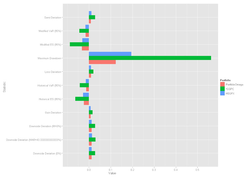
downsideTable<-melt(cbind(rownames(table.DownsideRisk(returnComparison)),table.DownsideRisk(returnComparison)))
colnames(downsideTable)<-c("Statistic","Portfolio","Value")
ggplot(downsideTable, stat="identity", aes(x=Statistic,y=Value,fill=Portfolio)) + geom_bar(position="dodge") + coord_flip()