Monday, July 11, 2011

Drawdown Control Can Also Determine Ending Wealth

As an extension to yesterday’s post Just Arriving is Not Enough, I wanted to show how minimizing drawdown is a much better technique to help control comfort and potentially increase ending wealth.  CHTTX was one of the best performers of the four funds OAKMX, CHTTX, FAIRX, and FCTNX mentioned in Smart Money “Bouncing Back with the World’s Greatest Investors.”  The fund suffered a brutal 60% drawdown though, and I’m guessing most of the original investors did not stick with the fund the entire time as the pain forced them out.  However, if we can limit the drawdown to something better than the excruciating 60%, then the ride is much smoother, or if someone truly is comfortable with 60% drawdown, we can apply leverage (I absolutely do not recommend) to both tailor the smoothness of our ride and also significantly increase ending wealth.

From TimelyPortfolio

We could apply up to 2.57 times leverage and incur the same drawdown as CHTTX, but let’s use a more conservative 2 times to see how it affects our simple system.

From TimelyPortfolio

In addition, if I as the money manager apply some drawdown control to my clients’ portfolio, I can help maintain their confidence and also significantly increase their ending wealth by not forcing them to make a decision based on fear.

R code (click to download):

#look at funds run by Smart Money's "world's greatest investors"
#http://www.smartmoney.com/invest/stocks/bouncing-back-with-the-worlds-greatest-investors-1309909342753/?cid=sm_dailyfinanceRSS
#then apply a simple moving average system
#to prove a point about controlling drawdown   require(quantmod)
require(PerformanceAnalytics)   tckr<-c("OAKMX","CHTTX","FAIRX","FCNTX")   start<-"1990-01-01"
end<- format(Sys.Date(),"%Y-%m-%d") # yyyy-mm-dd   # Pull tckr index data from Yahoo! Finance
getSymbols(tckr, from=start, to=end, adjust=TRUE)   RetToAnalyze<-merge(dailyReturn(OAKMX),dailyReturn(CHTTX),
dailyReturn(FAIRX), dailyReturn(FCNTX))
colnames(RetToAnalyze)<-tckr   #get very helpful Ken French data on Momentum Portfolios
#to compare to the funds
#http://mba.tuck.dartmouth.edu/pages/faculty/ken.french/ftp/6_Portfolios_ME_Prior_12_2_Daily.zip   my.url="http://mba.tuck.dartmouth.edu/pages/faculty/ken.french/ftp/6_Portfolios_ME_Prior_12_2_Daily.zip"
my.tempfile<-paste(tempdir(),"\\frenchmomentum.zip",sep="")
my.usefile<-paste(tempdir(),"\\6_Portfolios_ME_Prior_12_2_Daily.txt",sep="")
download.file(my.url, my.tempfile, method="auto",
quiet = FALSE, mode = "wb",cacheOK = TRUE)
unzip(my.tempfile,exdir=tempdir(),junkpath=TRUE)
#read space delimited text file extracted from zip
french_momentum <- read.table(file=my.usefile,
header = TRUE, sep = "",
as.is = TRUE,
skip = 12, nrows=12061)
colnames(french_momentum) <- c(paste("Small",
colnames(french_momentum)[1:3],sep="."),
paste("Large",colnames(french_momentum)[1:3],sep="."))   #get dates ready for xts index
datestoformat <- rownames(french_momentum)
datestoformat <- paste(substr(datestoformat,1,4),
substr(datestoformat,5,6),substr(datestoformat,7,8),sep="-")   #get xts for analysis
french_momentum_xts <- as.xts(french_momentum[,1:6],
order.by=as.Date(datestoformat))
#divide by 100 to get in decimal form
french_momentum_xts <- french_momentum_xts/100   #get column 3 for small momentum and 6 for large momentum
#to compare with the funds
RetWithFrench <-merge(RetToAnalyze,french_momentum_xts[,c(3,6)])   #jpeg(filename="performance summary of funds.jpg",quality=100,width=6.25, height = 8, units="in",res=96)
#charts.PerformanceSummary(RetWithFrench,ylog=TRUE,
# main="Smart Money World's Greatest Investors???",
# colorset=c("cadetblue","darkolivegreen3","goldenrod",
# "purple","gray","beige"))
#dev.off()   #let's just use a Mebane Faber style 200 day moving average
#to determine entry and exit
#for the best performer CHTTX
signal <- ifelse(CHTTX[,4]>runMean(CHTTX[,4],200),1,0)
signal <- merge(lag(signal,k=1),RetWithFrench[,2])
retCHTTX <- merge(signal[,1] * signal[,2], signal[,2])
colnames(retCHTTX) <- c("CHTTXMeanSystem","CHTTX")
#jpeg(filename="performance summary of chttx and mean system.jpg",quality=100,width=6.25, height = 8, units="in",res=96)
charts.PerformanceSummary(retCHTTX,ylog=TRUE,
main="Smart Money World's Greatest Investors???
CHTTX with 200 Day Mean System"
,
colorset=c("cadetblue","purple"))
#dev.off()   #if the investor is comfortable with 60% drawdown
#then they should be comfortable with leverage applied
#to the simple mean system; 2.57 would make them even
#in terms of max drawdown
#jpeg(filename="worst drawdown of chttx and mean system.jpg",quality=100,width=6.25, height = 8, units="in",res=96)
barplot(maxDrawdown(retCHTTX), main="Worst Drawdown Comparison",
ylim=c(0,0.6))
dev.off()
#print(maxDrawdown(retCHTTX[,2])/maxDrawdown(retCHTTX[,1]))   #let's see now what it looks like with just 2 times leverage
#applied to the simple mean system
retCHTTX <- merge(signal[,1] * signal[,2], signal[,1] * 2 * signal[,2], signal[,2])
colnames(retCHTTX) <- c("CHTTXMeanSystem","CHTTXMean2xLeverage","CHTTX")
#jpeg(filename="performance summary of chttx and mean system and leverage.jpg",quality=100,width=6.25, height = 8, units="in",res=96)
charts.PerformanceSummary(retCHTTX,ylog=TRUE,
main="Smart Money World's Greatest Investors???
CHTTX with 200 Day Mean System and 2x Leverage"
,
colorset=c("cadetblue","darkolivegreen3","purple"))
#dev.off()   #check max drawdown
#now by controlling drawdown we can end up with almost double the money
#with still less total drawdown
#jpeg(filename="worst drawdown of chttx and mean system with leverage.jpg",quality=100,width=6.25, height = 8, units="in",res=96)
barplot(maxDrawdown(retCHTTX), main="Worst Drawdown Comparison",
ylim=c(0,0.6))
#dev.off()
jpeg(filename="cumulative return of chttx and mean system with leverage.jpg",quality=100,width=6.25, height = 8, units="in",res=96)
barplot(Return.cumulative(retCHTTX), main="Cumulative Returns Comparison",
ylim=c(0,5))
dev.off()
print(Return.cumulative(retCHTTX[,2])/Return.cumulative(retCHTTX[,3]))

Created by Pretty R at inside-R.org

Sunday, July 10, 2011

Just Arriving is Not Enough

When you fly on an airplane, just arriving at your destination is not enough.  Almost all passengers want the ride to be super smooth and will sacrifice convenience and an on-time arrival to ensure comfort and perceived safety.  Also, passengers expect pilots to make this decision for them.  Like a pilot, I feel as a money manager, I bear the responsibility for the smoothness of my clients’ financial journey.  Unlike a pilot though, I have a much more significant burden since my clients can pull the emergency release as soon as they experience any discomfort.  Exiting due to panic or lack of confidence means my clients possibly make a financially fatal decision and either arrive late or never at their financial destination, so I must be even more cautious to not test the limits of my clients’ comfort.

When the ride is smooth, most of my clients do not care how fast I fly, but when the skies are unclear and the bumps severe, I need to take a different route (allocation) or not fly at all (sit in cash).  I would rather my client arrive a little late than to pull the emergency release and not arrive at all.  Pilots do not control the weather, and I do not control the markets, but we both must properly gauge conditions and make the decision to sacrifice convenience and an on-time arrival for a safe and comforable arrival.

Smart Money “Bouncing Back with the World’s Greatest Investors” does not seem to agree with my money management philosophy.  On the first manager Bill Nygren I see “Oakmark's 4 percent loss in 2007, and to a more dismal drop of 36 percent in 2008,” and these devastating drawdowns persist through the all four managers.  What troubles me most is how quickly the press and investors forgive pitiful performance and awful drawdowns in the crisis. These investors neither foresaw nor controlled the almost $10 trillion in political and monetary decisions required to temporarily rescue them. Here is a look at the mentioned funds.  Most of these managers simply avoided tech stocks in 2000-2003, but did nothing to avoid the far more severe disaster of 2007-2009.

From TimelyPortfolio

This is unacceptable to me, and I believe the flawed forgiveness will be punished in the next cycle as these managers, their investors, and the press learned nothing from the last crisis.

R code (click to download):

#look at funds run by Smart Money's "world's greatest investors"
#http://www.smartmoney.com/invest/stocks/bouncing-back-with-the-worlds-greatest-investors-1309909342753/?cid=sm_dailyfinanceRSS   require(quantmod)
require(PerformanceAnalytics)   tckr<-c("OAKMX","CHTTX","FAIRX","FCNTX")   start<-"1990-01-01"
end<- format(Sys.Date(),"%Y-%m-%d") # yyyy-mm-dd   # Pull tckr index data from Yahoo! Finance
getSymbols(tckr, from=start, to=end, adjust=TRUE)   RetToAnalyze<-merge(dailyReturn(OAKMX),dailyReturn(CHTTX),
dailyReturn(FAIRX), dailyReturn(FCNTX))
colnames(RetToAnalyze)<-tckr   #get very helpful Ken French data on Momentum Portfolios
#to compare to the funds
#http://mba.tuck.dartmouth.edu/pages/faculty/ken.french/ftp/6_Portfolios_ME_Prior_12_2_Daily.zip   my.url="http://mba.tuck.dartmouth.edu/pages/faculty/ken.french/ftp/6_Portfolios_ME_Prior_12_2_Daily.zip"
my.tempfile<-paste(tempdir(),"\\frenchmomentum.zip",sep="")
my.usefile<-paste(tempdir(),"\\6_Portfolios_ME_Prior_12_2_Daily.txt",sep="")
download.file(my.url, my.tempfile, method="auto",
quiet = FALSE, mode = "wb",cacheOK = TRUE)
unzip(my.tempfile,exdir=tempdir(),junkpath=TRUE)
#read space delimited text file extracted from zip
french_momentum <- read.table(file=my.usefile,
header = TRUE, sep = "",
as.is = TRUE,
skip = 12, nrows=12061)
colnames(french_momentum) <- c(paste("Small",
colnames(french_momentum)[1:3],sep="."),
paste("Large",colnames(french_momentum)[1:3],sep="."))   #get dates ready for xts index
datestoformat <- rownames(french_momentum)
datestoformat <- paste(substr(datestoformat,1,4),
substr(datestoformat,5,6),substr(datestoformat,7,8),sep="-")   #get xts for analysis
french_momentum_xts <- as.xts(french_momentum[,1:6],
order.by=as.Date(datestoformat))
#divide by 100 to get in decimal form
french_momentum_xts <- french_momentum_xts/100   #get column 3 for small momentum and 6 for large momentum
#to compare with the funds
RetWithFrench <-merge(RetToAnalyze,french_momentum_xts[,c(3,6)])     jpeg(filename="performance summary of funds.jpg",quality=100,width=6.25, height = 8, units="in",res=96)
charts.PerformanceSummary(RetWithFrench["2003-03::2011-05",],ylog=TRUE,
main="Smart Money World's Greatest Investors???",
colorset=c("cadetblue","darkolivegreen3","goldenrod",
"purple","gray","beige"))
dev.off()

Created by Pretty R at inside-R.org

Thursday, July 7, 2011

Scary Derivatives and Scary XML in R

I need some new R skills, and there is no better motivation to learn XML in R than one of the scariest financial datasets out there—the US Department of the Treasury Office of the Comptroller of the Currency (OCC) Quarterly Derivatives Report. I’ll move to the even scarier global BIS derivatives data in a later post to avoid inducing nightmares and sleepless nights.

The massive damage caused in 2008-2009 by the sliver of derivatives called credit default swaps seems like a faint warning siren when we see that they only represent < 7% of total derivatives exposure.  Interest rate and currency derivatives, also where I think the next disaster occurs, are more than 10 times larger than these credit contracts at $226 Trillion.  While some take comfort in

“Bilateral Netting: A legally enforceable arrangement between a bank and a counterparty that creates a single legal obligation covering all included individual contracts. This means that a bank‟s receivable or payable, in the event of the default or insolvency of one of the parties, would be the net sum of all positive and negative fair values of contracts included in the bilateral netting arrangement.”

bilateral netting does not work so well when your counterparty fails like Lehman Brothers.

From TimelyPortfolio

I know there must be a better way to read Microsoft Excel XML spreadsheets in R, but these were my two most elegant methods.  Please let me know how I could have done better.

R code (click to download):

#read xml derivatives data from the
#US Treasury OCC Quarterly Derivatives Report
#2 methods of as far as I can tell
#the first published example of how to read
#Microsoft Excel xml workbooks   require(XML)
require(ggplot2)   url = "http://www.occ.treas.gov/topics/capital-markets/financial-markets/trading/derivatives/dq410-xml.xml"
#url = "dq410-xml.xml"   doc = xmlInternalTreeParse("dq410-xml.xml")
#define namespaces
#figuring this out took hours
#but using getNodeSet was much cleaner than the
#next method
namespaces = c(o="urn:schemas-microsoft-com:office:office",
x="urn:schemas-microsoft-com:office:excel",
ss="urn:schemas-microsoft-com:office:spreadsheet",
html="http://www.w3.org/TR/REC-html40")
ns <- getNodeSet(doc,"/ss:Workbook/ss:Worksheet[@ss:Name='Table 3']/ss:Table/ss:Row",namespaces)[[44]]
pct <- df <- as.data.frame(as.numeric(xmlSApply(ns, xmlValue))[5:8])
ns <- getNodeSet(doc,"/ss:Workbook/ss:Worksheet[@ss:Name='Table 3']/ss:Table/ss:Row",namespaces)[[8]]
lab <- as.character(xmlSApply(ns, xmlValue)[8:11])
df <- cbind(lab,df)
#jpeg(filename="derivatives by type.jpg",quality=100,
# width=6.25, height = 8, units="in",res=96)
barplot(df[,2],names.arg = df[,1],main="US Bank Derivatives by Type
Q4 2010"
,ylab="% of Total")
mtext("Source: US Dept of Treasury OCC Quarterly Derivatives Report",
side=1,line=3,cex=0.8,adj=0)
#dev.off()       #here is the original very hacked brute force method
doc = xmlRoot(xmlTreeParse(url))
#set xmlNodeList to Table 3
#hacked with brute force
table3 <- doc[6]$Worksheet
df <- as.data.frame(cbind(
as.numeric(
xmlApply(table3[[1]],function(x) xmlApply(x,xmlValue))[53]$Row[5:8])),
stringsAsFactors=FALSE)
df <- cbind(
as.character(xmlApply(table3[[1]],function(x) xmlApply(x,xmlValue))[17]$Row[c(8:11)]),
df)
colnames(df) <- c("DerivativeType","PctOfTotal")
barplot(df[,2],names.arg = df[,1],main="US Bank Derivatives by Type
Q4 2010"
,ylab="% of Total")
mtext("Source: US Dept of Treasury OCC Quarterly Derivatives Report",
side=1,line=3,cex=0.8,adj=0)

Created by Pretty R at inside-R.org

Tuesday, July 5, 2011

A Quantstrat to Build On Part 6

THIS IS NOT INVESTMENT ADVICE.  ACTING ON THIS MAY LOSE LOTS OF MONEY.

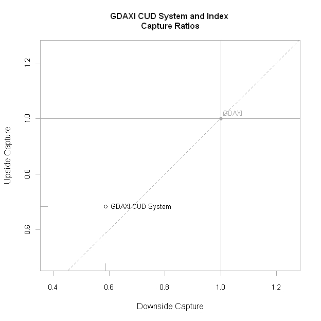
In A Quantstrat to Build on Part 5, I promised some performance reporting on quantstrat portfolios, but then in REIT Momentum in Quantstrat, I discovered it is not nearly as easy as I thought.  With some help from experts (please tell me if you would like me to mention you by name), I found a couple of ways to accomplish this crucial component of systems development.  We’ll compare the original simple CUD system with buy and hold but this time using the osFUN option in our entry rule to buy an amount equal to the proceeds from the previous trade.  Minimizing drawdown on the way down allows potentially larger trade quantities on the way back up.

From TimelyPortfolio

R code (click to download):

#thanks so much to the developers of quantstrat
#99% of this code comes from the demos in the quantstrat package   #in this I use osFun to size orders to ending equity
#for a more appropriate comparison to buy hold   #takes longer than I would like but is acceptable
#another way to accomplish testing and reporting
#is use 1 for orderqty and then generate return series
#with this as signal   #however despite extra time I like to see growth in order size
#with performance
#makes a very valid point for drawdown reduction     require(quantstrat)
require(PerformanceAnalytics)   #now let's define our silly countupdown function
CUD <- function(price,n) {
#CUD takes the n-period sum of 1 (up days) and -1 (down days)
temp <- runSum(ifelse(ROC(price,1,type="discrete") > 0,1,-1),n)
colnames(temp) <- "CUD"
temp
}   BuyHold <- function(price,periodtobuy) {
#just enter true (1) the period specified as buy and hold
#for the remainder
temp <- as.xts(rep(0,NROW(price)),order.by=index(price))
colnames(temp) <- "BuyHold"
temp[periodtobuy,1]<-1
temp
}   osFillErUp <- function (data, timestamp, orderqty, ordertype, orderside, portfolio, symbol, ruletype, ..., orderprice)
{   #get date in usable xts format
datePos <- format(timestamp,"%Y-%m-%d")
#update the portfolio to date of trade rule
updatePortf(Portfolio=portfolio,Symbol=symbol,Dates=paste('::',datePos,sep=''))
portf <- getPortfolio(portfolio)
#get price of symbol for the date of trade rule
price <- getPrice(get(symbol))[datePos]
#get amount generated from the last trade
#best way for me to overcome lack of cumulative p/l for portfolio by symbol
#all this logic is at the account level
trades <- getOrderBook(portfolio)[[portfolio]][[symbol]]
#if first trade, just use order quantity specified
#if not get order quantity equal to
#last trade proceeds divided by price of symbol at trade date
if(NROW(trades)>1) {
trades <- trades[NROW(trades)]
endEq <- as.numeric(trades$Order.Qty) * as.numeric(trades$Order.Price)
# orderqty <- abs(endEq/price)
orderqty <- abs(floor(endEq/price))
}
#return the new orderqty
osFillErUp <- orderqty
}     try(rm("order_book.CUD",pos=.strategy),silent=TRUE)
try(rm("order_book.BuyHold",pos=.strategy),silent=TRUE)
try(rm("account.CUD","portfolio.CUD",pos=.blotter),silent=TRUE)
try(rm("account.BuyHold","portfolio.BuyHold",pos=.blotter),silent=TRUE)
try(rm("port.st","symbols","symbol","stratCUD","initDate","initEq",
'start_t','end_t','num_periods'),silent=TRUE)   #specify this for the rolling periods to use for our signal
num_periods=50   # Initialize a strategy object
stratCUD <- strategy("CUD")   # Add an indicator
stratCUD <- add.indicator(strategy = stratCUD, name = "CUD",
arguments = list(price = quote(Cl(mktdata)),n=num_periods),
label="CUD")   # enter when CUD > 0
stratCUD <- add.signal(strategy = stratCUD, name="sigThreshold",
arguments = list(threshold=0, column="CUD",relationship="gte", cross=TRUE),
label="CUD.gte.0")
# exit when CUD < 0
stratCUD <- add.signal(strategy = stratCUD, name="sigThreshold",
arguments = list(threshold=0, column="CUD",relationship="lt",cross=TRUE),
label="CUD.lt.0")   stratCUD <- add.rule(strategy = stratCUD, name='ruleSignal',
arguments = list(sigcol="CUD.gte.0", sigval=TRUE, orderqty=100, ordertype='market',
orderside='long', pricemethod='market', replace=FALSE, osFUN='osFillErUp'), type='enter', path.dep=TRUE)
stratCUD <- add.rule(strategy = stratCUD, name='ruleSignal',
arguments = list(sigcol="CUD.lt.0", sigval=TRUE, orderqty='all',
ordertype='market', orderside='long', pricemethod='market', replace=FALSE),
type='exit', path.dep=TRUE)   #Initialize a buy/hold strategy object
stratBuyHold <- strategy("BuyHold")
stratBuyHold <- add.indicator(strategy = stratBuyHold, name = "BuyHold",
arguments = list(price = quote(Cl(mktdata)),periodtobuy=num_periods),
label = "BuyHold")
stratBuyHold <- add.rule(strategy=stratBuyHold, name='ruleSignal',
arguments = list(sigcol="BuyHold",sigval=TRUE,orderqty=100,ordertype='market',
orderside='long', pricemethod='market', replace=FALSE), type='enter', path.dep=TRUE)     currency("USD")
symbols = c("GSPC","GDAXI")
for (symbol in symbols) {
stock(symbol, currency="USD",multiplier=1)
#use paste with ^ to get index data
getSymbols(paste("^",symbol,sep=""),adjust=T,from="1900-12-31")
assign(symbol,to.weekly(get(symbol)))
}   initDate='1949-12-31'
initEq=1000000
port.st<-'CUD' #use a string here for easier changing of parameters and re-trying
port.buyhold <- 'BuyHold'   initPortf(port.st, symbols=symbols, initDate=initDate)
initAcct(port.st, portfolios=port.st, initDate=initDate, initEq=initEq)
initOrders(portfolio=port.st, initDate=initDate)   initPortf(port.buyhold, symbols=symbols, initDate=initDate)
initAcct(port.buyhold, portfolios=port.buyhold, initDate=initDate,, initEq=initEq)
initOrders(portfolio=port.buyhold, initDate=initDate)   print("setup completed")   # Process the indicators and generate trades
start_t<-Sys.time()
out<-try(applyStrategy(strategy=stratCUD , portfolios=port.st ) )
end_t<-Sys.time()
print("Strategy Loop:")
print(end_t-start_t)   # Process buy and hold strategy
start_t<-Sys.time()
out<-try(applyStrategy(strategy=stratBuyHold , portfolios=port.buyhold ) )
end_t<-Sys.time()
print("Strategy Loop:")
print(end_t-start_t)   start_t<-Sys.time()
updatePortf(Portfolio=port.st,Dates=paste('::',as.Date(Sys.time()),sep=''))
updatePortf(Portfolio=port.buyhold,Dates=paste('::',as.Date(Sys.time()),sep=''))
end_t<-Sys.time()
print("trade blotter portfolio update:")
print(end_t-start_t)   # hack for new quantmod graphics, remove later
themelist<-chart_theme()
themelist$col$up.col<-'lightgreen'
themelist$col$dn.col<-'pink'   for(symbol in symbols){
#dev.new()
#chart.Posn(Portfolio=port.st,Symbol=symbol,theme=themelist)
#add the CUD indicator to the bottom of the chart
#jpeg(filename=paste(symbol," Reconcile.jpg",sep=""),quality=100,
# width=6.5, height = 6.5, units="in",res=96)
chart.Reconcile(port.buyhold,port.st,symbol)
plot(add_TA(CUD(get(symbol)[,4],n=num_periods)))
#dev.off()
}   #tradeStats(port.st)   #backwards way to get returns
#again to bypass account p/l logic
port <- getPortfolio(port.st)
for(symbol in symbols) {
#get posPL for the symbol in the portfolio
posPLTable <- port$symbols[[symbol]][["posPL"]]
#easier this way to get ROC for each day when position is held (Pos.Qty > 0)
#rets <- lag(ifelse(posPLTable$Pos.Qty>0,1,0),k=1)*ROC(get(symbol)[,4],type="discrete",n=1)
#the previous commented method is not exactly correct
#since we can only hold integer positions
#to account for this difference we can get
rets <- posPLTable$Gross.Trading.PL/lag(posPLTable$Pos.Value,k=1)
rets[is.na(rets)] <- 0
rets[which(rets[,1]==Inf)] <- 0
rets[which(rets[,1]==-Inf)] <- 0
retCompare <- merge(rets,ROC(get(symbol)[,4],type="discrete",n=1))
colnames(retCompare) <- c(paste(symbol," CUD System",sep=""),symbol)
#jpeg(filename=paste(symbol," Performance.jpeg",sep=""),quality=100,width=6.5, height = 6.5,
# units="in",res=96)
charts.PerformanceSummary(retCompare,ylog=TRUE,
colorset=c("black","gray70"),
main = paste(symbol," CUD System and Index
Performance Summary"
,sep=""))
#dev.off()
#jpeg(filename=paste(symbol," Capture.jpeg",sep=""),quality=100,width=6.5, height = 6.5,
# units="in",res=96)
chart.CaptureRatios(retCompare[,1],retCompare[,2],
main = paste(symbol," CUD System and Index
Capture Ratios"
,sep=""))
#dev.off()
}

Created by Pretty R at inside-R.org