Showing posts with label javascript. Show all posts

Tuesday, July 26, 2016

Ooms Magical Polyglot World

crossposted from BuildingWidgets

Jeroen Ooms (@opencpu) provides R users a magical polyglot world of R, JavaScript, C, and C++. This is my attempt to both thank him and highlight some of all that he has done. Much of my new R depends on his work.

Ooms' Packages

metacran provides a list of all Jeroen's CRAN packages. Now, I wonder if any of his packages are in the Top Downloads.

jsonlite

Let's leverage the helpful meta again from metacran and very quickly get some assistance from hint-hint jsonlite.

library(jsonlite)
library(formattable)
library(tibble)
library(magrittr)

fromJSON("http://cranlogs.r-pkg.org/top/last-month/9") %>%
  {as_tibble(rank=rownames(.$downloads),.$downloads)} %>%
  rownames_to_column(var = "rank") %>%
  format_table(
    formatters = list(
      area(row=which(.$package=="jsonlite")) ~ formatter("span", style="background-color:#D4F; width:100%")
    )
  )
rank package downloads
1 Rcpp 236316
2 plyr 208609
3 ggplot2 201959
4 stringi 188252
5 jsonlite 175853
6 digest 174714
7 stringr 173835
8 magrittr 166437
9 scales 156694
`jsonlite` is an ultra-fast reliable tool to convert and create `json` in `R`. It's fast because like much Jeroen's work, he leverages `C`/`C++` libraries. `shiny` and `htmlwidgets` both depend on `jsonlite`.

V8

V8 gives R its own embedded JavaScript engine to leverage functionality in JavaScript that might not exist in R. For example, the WebCola constraint-based layout engine offers valuable technology not available within R. Let's partially recreate the smallgroups example all in R. You might notice that the previously mentioned jsonlite is essential to this workflow.

library(V8)
library(jsonlite)
library(scales)

ctx = new_context(global="window")

ctx$source("https://cdn.rawgit.com/tgdwyer/WebCola/master/WebCola/cola.min.js")

## [1] "true"

### small grouped example
group_json <- fromJSON(
  system.file(
    "htmlwidgets/lib/WebCola/examples/graphdata/smallgrouped.json",
    package = "colaR"
  )
)

# need to get forEach polyfill
ctx$source(
  "https://cdnjs.cloudflare.com/ajax/libs/es5-shim/4.1.10/es5-shim.min.js"
)

# code to recreate small group example
js_group <- '
// console.assert does not exists
console = {}
console.assert = function(){};

var width = 960,
  height = 500

graph = {
"nodes":[
  {"name":"a","width":60,"height":40},
  {"name":"b","width":60,"height":40},
  {"name":"c","width":60,"height":40},
  {"name":"d","width":60,"height":40},
  {"name":"e","width":60,"height":40},
  {"name":"f","width":60,"height":40},
  {"name":"g","width":60,"height":40}
],
"links":[
  {"source":1,"target":2},
  {"source":2,"target":3},
  {"source":3,"target":4},
  {"source":0,"target":1},
  {"source":2,"target":0},
  {"source":3,"target":5},
  {"source":0,"target":5}
],
"groups":[
  {"leaves":[0], "groups":[1]},
  {"leaves":[1,2]},
  {"leaves":[3,4]}
  ]
}

var g_cola = new cola.Layout()
  .linkDistance(100)
  .avoidOverlaps(true)
  .handleDisconnected(false)
  .size([width, height]);

g_cola
  .nodes(graph.nodes)
  .links(graph.links)
  .groups(graph.groups)
  .start()
'

# run the small group JS code in V8
ctx$eval(js_group)

## [1] "[object Object]"

Now, WebCola has done the hard work and laid out our nodes and links, so let's get their positions.

nodes <- ctx$get('
  graph.nodes.map(function(d){
    return {name: d.name, x: d.x, y: d.y, height: d.height, width: d.width};
  })
')

links <- ctx$get('
  graph.links.map(function(d){
    return {x1: d.source.x, y1: d.source.y, x2: d.target.x, y2: d.target.y}
  })
')

Some great examples of packages employing V8 are geojsonio, lawn, DiagrammeRsvg, rmapshaper, and daff.

rjade

We got layout coordinates above. Let's use another one of Jeroen's packages rjade that provides jade (now called pug) templates through V8. rjade will let us build a SVG graph with our layout.

library(rjade)
library(htmltools)

svg <- jade_compile(
'
doctype xml
svg(version="1.1",xmlns="http://www.w3.org/2000/svg",xmlns:xlink="http://www.w3.org/1999/xlink",width="960px",height="500px")
  each l in lines
    line(style={fill:none, stroke:"lightgray"})&attributes({"x1": l.x1, "x2": l.x2, "y1": l.y1, "y2": l.y2})
  each val in rects
    g
      rect(style={fill: fillColor})&attributes({"x": val.x - val.width/2, "y": val.y - val.height/2, "height": val.height - 6, "width": val.width - 6, rx: 5, ry: 5})
      text&attributes({"x": val.x, "y": val.y, "dy": ".2em", "text-anchor":"middle"})= val.name
'
      ,pretty=T
)(rects = nodes, lines = links, fillColor = "lightgray")

HTML(svg)
a b c d e f g

rsvg

If we are not in the browser though with inline SVG support, we very likely will want a static image format such as png or jpeg. Of course, Jeroen has that covered also with the crazy-speedy rsvg. Jeroen offers base64, but in this case we will use base64enc, since it allows raw.

library(rsvg)
library(base64enc)

graph_png <- rsvg_png(charToRaw(svg))

tags$img(src=dataURI(graph_png), mime="image/png")

magick

Jeroen's newest package magick is in my mind the coolest. magick gives us all the power of ImageMagick as easy R functions, and is pure wizardry. I am still shocked that it compiled first try with absolutely no problems.

library(magick)

graph_img <- image_read(graph_png)
wizard_img <- image_read("http://www.imagemagick.org/image/wizard.png")

images <- image_annotate(
  image_append(
    c(
      image_scale(image_crop(wizard_img, "600x600+100+100"), "100"),
      image_crop(graph_img, "400x400+200+0")
    )
  ),
  "Ooms is a Wizard!",
  size = 20,
  color = "blue",
  location = "+100+200"
)

tags$img(src=dataURI(image_write(images)), mime="image/png")

commonmark

I should note that this document was assembled in rmarkdown. RStudio gives us lots of tools for working with rmarkdown, but Jeroen gives us a powerful tool commonmark. Let's use it to give our readers other options for output.

library(commonmark)

rmarkdown::render("Readme.Rmd", "Readme.md", output_format="md_document")

tex <- markdown_latex(readLines("Readme.md"))
cat(tex, file="Readme.tex")

This would convert markdown to LaTeX. As a test, I used commonmark to make the html for this post.

Conclusion and Thanks

There are of course more packages, but I'll stop here. Jeroen Ooms truly is a wizard, and the R community is extraordinarily blessed to have him. Thanks so much Jeroen.

For even more wizardry, be sure to check out opencpu from Jeroen, which makes R available as a web service.

Wednesday, March 11, 2015

Extracting Heatmap

Inspired by this tweet, I wanted to try to do something similar in JavaScript.

Fortunately, I had this old post Chart from R + Color from Javascript to serve as a reference, and I got lots of help from these links.

In a couple of hours, I got this crude but working rendering complete with a d3.js brush to get the scale.  Then since this is sort of a finance blog, I imagined we found an old correlation heatmap like the one in Pretty Correlation Map of PIMCO Funds.  Although, we could guess at the correlation values, I thought it would be a lot more fun to get live values.  Try it out below.

  1. Brush over the scale / legend
  2. Input scale min and max
  3. Mouseover color areas in the chart

As I said, it is rough, but it works. It needs a little UI work :)

Tuesday, December 30, 2014

Widgets For Christmas

For Christmas, I generally want electronic widgets, but after six months of development, all I wanted this Christmas was htmlwidgets, and Santa RStudio/jj,joe,yihui and Santa Ramnath delivered early with this RStudio tweet on December 17th.

The major benefit of htmlwidgets is it provides all three methods of bridging R with JavaScript/HTML mentioned in my Aug. 16, 2013 post I Want ggplot2/lattice and d3 (gridSVG–The Glue).  For htmlwidgets to be successful though, not only do htmlwidgets need to work, easy creation of widgets is absolutely essential.

As a quick example, we can look at the DiagrammeR package released yesterday by Richard Iannone.  DiagrammeR launched in non-htmlwidgets form severely hampering its ability to be easily used in multiple contexts.  Converting it to htmlwidgets seemed like a great opportunity to illustrate both the ease of htmlwidgets creation and the powerful infrastructure offered by htmlwidgets.  So, in a couple hours—easy to create, check—yesterday (most of the time spent on examples, documentation, and testing) with only a couple of lines of JavaScript—easy to create, check again—I was able to transform the DiagrammeR package into htmlwidgets.

I thought a finance diagram would be a great example for this blog, so off to Google Images I went looking for a good and also simple application and chose this from the Department of Finance Canada.

image

Here is what it looks like with DiagrammeR + mermaid.js.


If I can come up with the resolve and commitment, I might have an announcement for 2015 – the year of the widget.

Happy New Year, and thanks for 4 good years of TimelyPortfolio.

Friday, October 10, 2014

SVG + Javascript Ekholm Decomposition in RStudio Browser

Our topics this week seem unrelated, but in an effort to bridge the two

another random project – make website in R for these SVGs of Portland Vector Bridges
result: Portland Bridges in SVG
code: R to make simple site

Ekholm decomposition

SelectionShare & TimingShare | Masterfully Written by Delightfully Responsive Author
Popular Mutual Funds Decomposed With Ekholm (2014)

Responsive SVG in the browser

Responsive SVG in Your RStudio Browser
SVG + a little extra (d3.js) in RStudio Browser | No Pipes This Time

let’s build a website in R with htmltools to calculate the Ekholm decomposition in Javascript using this nifty simple-statistics.js from the brilliant Tom Macwright.  The result will not be beautiful and I’ll leave out a fancy interactive chart, but that is intentional to reduce the amount of code and dependencies.

r_ekholm_js

I wonder what I’ll get into next week.

Github Repo

library(htmltools)
library(pipeR)
library(jsonlite)
library(Quandl)
library(xts)

# use Quandl Kenneth French Fama/French factors
# http://www.quandl.com/KFRENCH/FACTORS_D
#f <- Quandl("KFRENCH/FACTORS_D",type = "xts", start_date="2010-12-31") / 100

tagList(
#pull in the bridge to span all the week's topics
#Portland Vector Bridges http://timelyportfolio.github.io/portland_vector_bridges
tags$div( style = "height:15%;width:100%"
,readLines(
"http://timelyportfolio.github.io/portland_vector_bridges/Burnside Bridge.svg"
) %>>% HTML
)
,tags$h1( "Sparsest Test in Javascript of Ekholm")
, tags$div( style = "width:100%"
,tags$div( style = "background-color:red;"
,"Note: Date range currently limited to one year, but there is a fairly easy workaround
for the next version."
)
,tags$div(
style = "display:inline-block; width: 25%;float:left;"
,"Mutual Fund Symbol", tags$input( id = "mfsymbol" )
,tags$br()
,"Start Date "
, tags$span( style="font-size:75%;fill:lightgray", "(2013-08-29)" )
, tags$input( type = "date", id = "stdate" )
,tags$br()
,"End Date"
,tags$span( style="font-size:75%;fill:lightgray", "(2014-08-29)" )
, tags$input( type = "date", id= "enddate" )
,tags$br()
,tags$input(
type="submit", id = "calc", value = "Calculate"
)
,tags$br()
)
, tags$div(style = "display:inline-block;height:100%;width:60%;margin-left:30px"
, tags$textarea(id = "results", style="width:100%; height:150px")
)
)
,tags$script(sprintf(
'

var french = %s;
'
, toJSON(data.frame("Date"=index(f),f)) %>>% HTML
))
,tags$script(
'

function calculateEkholm( data ) { // data in form of x,y or fund-rf, mkt-rf
/* get an error with regression.js
var myReg = regression(
"linear",
data
)
*/

// so use the great simple-statistics library
var myReg = ss.linear_regression().data(data);

//get residuals
var resid = data.map(function(p){return myReg.line()(p[0]) - p[1]});

//regress residuals^2 on (mkt-rf)^2
var myReg2 = ss.linear_regression().data(
data.map(function(d,i){
return [ Math.pow(d[0],2), Math.pow(resid[i],2) ]
})
)
//coefficients ^ 1/2 will give us ActiveAlpha and ActiveBeta
var activeAlpha = Math.pow( myReg2.b(), 0.5 );
var activeBeta = Math.pow( myReg2.m(), 0.5 );

//now do the next step to get ActiveShare and SelectionShare
var selectionShare = Math.pow(activeAlpha, 2 ) / ( ss.variance(data.map(function(d){return d[1]})) * (data.length - 1) / data.length )
var timingShare = Math.pow(activeBeta, 2 ) * ss.mean( data.map(function(d){return Math.pow(d[0],2)}) ) / ( ss.variance(data.map(function(d){return d[1]})) * (data.length - 1) / data.length )

//pass correlation result also
var correlation = ss.sample_correlation(data.map(function(d){return d[0]}),data.map(function(d){return d[1]}));

return {
regression: myReg,
correlation: correlation,
activeAlpha: activeAlpha,
activeBeta: activeBeta,
selectionShare: selectionShare,
timingShare: timingShare
}
}


// thanks https://gist.github.com/fincluster/6145995
function getStock(opts, type, complete) {
var defs = {
desc: false,
baseURL: "http://query.yahooapis.com/v1/public/yql?q=",
query: {
quotes: \'select * from yahoo.finance.quotes where symbol = \"{stock}\" | sort(field=\"{sortBy}\", descending=\"{desc}\")\',
historicaldata: \'select * from yahoo.finance.historicaldata where symbol = \"{stock}\" and startDate = \"{startDate}\" and endDate = \"{endDate}\"\'
},
suffixURL: {
quotes: "&env=store://datatables.org/alltableswithkeys&format=json&callback=?",
historicaldata: "&env=store://datatables.org/alltableswithkeys&format=json"
}
};

opts = opts || {};

if (!opts.stock) {
complete("No stock defined");
return;
}

var query = defs.query[type]
.replace("{stock}", opts.stock)
.replace("{sortBy}", defs.sortBy)
.replace("{desc}", defs.desc)
.replace("{startDate}", opts.startDate)
.replace("{endDate}", opts.endDate)

var url = defs.baseURL + query + (defs.suffixURL[type] || "");

return url;
}


d3.select("#calc").on("click",function(){
calculateFund(
d3.select("#mfsymbol")[0][0].value,
d3.select("#stdate")[0][0].value,
d3.select("#enddate")[0][0].value
)
})

function calculateFund( symbol, startdate, enddate ) {

d3.json(getStock({stock:symbol.toUpperCase(),startDate:startdate,endDate:enddate},"historicaldata"), function(e1,fund){


if( e1 || !fund.query.results ) {
updateResults ( {e1:e1, e2:e2, queryresults: "query problems"} );
} else {
var fund_factor = [];

//manipulate data to join fund with factors
//would be nice to have a xts merge in javascript


// query.results.quote will have the data stripped of meta
// also we will sort date ascending
fund = fund.query.results.quote
.sort(function(a,b){
return d3.ascending(
d3.time.format("%Y-%m-%d").parse(a.Date),
d3.time.format("%Y-%m-%d").parse(b.Date)
)
} );


// now lets go period by period with fund.map
fund.map( function(per, i){
if( i > 0 ) {
var frenchThisPer = french.filter(function(d){return d.Date == per.Date})[0];
fund_factor.push([
//Date: per.Date,
//FundPrice:
per.Adj_Close / fund[ i - 1 ].Adj_Close - 1 - frenchThisPer["RF"],
//Rm_Rf:
+frenchThisPer["Mkt.RF"],
//Rf: +frenchThisPer["RF"]/100
])
}
})

updateResults( calculateEkholm( fund_factor ) );
}

})
}

function updateResults( ekholmCalc ){
var ekhArr = [];
Object.keys(ekholmCalc).map(function(k){
ekhArr.push( [ k,": ", ekholmCalc[k] ].join("") )
})
d3.select("#results").text(ekhArr.join("\\n"))
}
'
%>>% HTML )
) %>>%
attachDependencies(
list(
htmlDependency(
name="d3"
,version="3.4"
,src=c("href"="http://d3js.org/")
,script="d3.v3.min.js"
)
,htmlDependency(
name="simple_statistics"
,version="0.1"
,src=c("href"=
"http://timelyportfolio.github.io/rCharts_factor_analytics/js"
)
,script = "simple_statistics.js"
)
)
) %>>% html_print

Tuesday, July 22, 2014

Chart from R + Color from Javascript

Another color experiment combining resources from R and Javascript.  I just wish I could do Mean Phylogenetic Distance in Javascript like rPlotter.  I enjoyed using d3.js zoom behavior to pan and zoom the image on canvas.  Also, filedrop.js made the drag and drop image easy.  There are lots of mini lessons in this code for someone who want to pick inside the code.

You might also notice the reference color from my last post Pick a Color Site built in R with Shiny tags %$%.

image

Tuesday, March 25, 2014

Interactive Discovery of Research Affiliates JoPM Paper

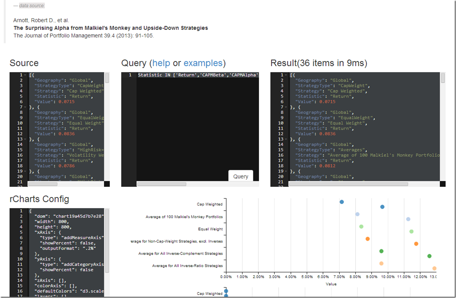
In my previous post More on Rebalancing | With Data from Research Affiliates , I did some really basic visualizations, but I thought this data would be great for some more powerful interactive discovery using an interesting javascript SQL-like query language objeq along with the d3.js charting library dimple.js.  Next, I hope to extend to use lodash or lazy.js.

This exercise helps me think through a couple of lingering issues:

  1. After we create the plot, do we need to maintain the overhead of a connection with R using something like shiny, or can we port some of the aggregation, filtering, and calculations to javascript as we did in this example?
  2. How can we use the rCharts templates with other languages such as Python, Ruby, and Javascript?
  3. What can we do with some more specific and customized page templates for rCharts?
  4. Is a Lyra-like interface better or will this type interface work for more advanced users?

Help me with your thoughts after you have played with the example shown by the screenshot below.image

Wednesday, November 27, 2013

Something to Think About Before Black Friday | rChart + dygraphs

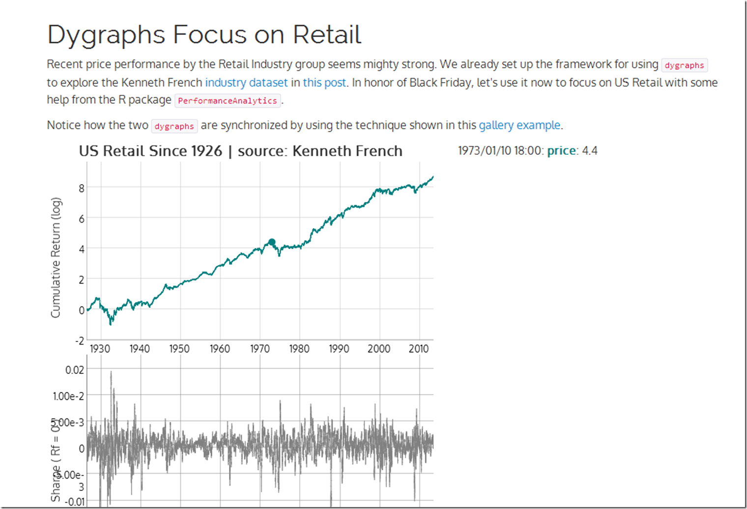
US Retail stocks have been killing it.  Since the holiday season starting with Black Friday is so important to retail, let’s look at the US Retail industry price and Sharpe ratio using R rCharts and Performance analytics +  javascript dygraphs.  Thanks Kenneth French once again for the dataset.

image

Friday, November 15, 2013

Dygraphs with Bigger Data | US Industries from Kenneth French

After seeing the announcement by @lauraegerdal of the SEC’s use of dygraphs to visualize market structure, I was inspired to experiment more with the great dygraphs + rCharts.  I really wanted to see how responsive dygraphs would be with a fairly large dataset.  Some Kenneth French US Industry data seemed just big enough to get a good feel for dygraph’s digestive abilities.  See it in action here or click on the screenshot below.

image

Wednesday, August 28, 2013

Applications of Interactivity to Finance

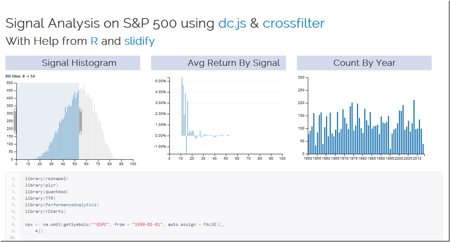
Of the nearly infinite ways of using crossfilter and dc.js in finance, the 2 that immediately came to my mind are signal analysis in system building and money manager analysis in due diligence.  My first very basic experiment explores a commonly known signal (RSI) on the daily S&P 500 since 1950.  Interactivity adds a lot to the experience.  I used R to grab and reshape the data and slidify to make it pretty.  Check it out by clicking here or on the screenshot below.

screenshot

For another very fine example of dc.js and crossfilter in use with AAII Stockpicking strategy data, see this fine site.

image

Wednesday, August 7, 2013

ggplot2 meet d3

With great libraries, just a couple lines of code can do amazing things.  For instance, let’s limit ourselves to less than 10 lines of code and see what ggplot2 and d3 can do.  We will use gridSVG as discussed in yesterday’s post I Want ggplot2/lattice and d3 (gridSVG–The Glue) to expose ggplot2 to d3.  Thanks Hadley Wickham, Mike Bostock, Paul Murrell, Simon Potter, and George Bull/Sharp Statistics.

If the iframe does not appear below, click here.

Just think what we can do if we remove our 10 line code limit.

#get the latest version of gridSVG
#install.packages("gridSVG", repos="http://R-Forge.R-project.org")

require(ggplot2)
require(gridSVG)

#draw a ggplot2 graph
#thanks http://sharpstatistics.co.uk/r/ggplot2-guide/
p <- ggplot(iris, aes(Sepal.Length, Sepal.Width)) + geom_point()
p + facet_grid(. ~ Species) + stat_smooth(method = "lm")

#define a simple html head template
htmlhead <-
'<!DOCTYPE html>
<head>
<meta charset = "utf-8">
<script src = "http://d3js.org/d3.v3.js"></script>
</head>

<body>
'


#use gridSVG to export our plot to SVG
mysvg <- grid.export("panzoom1.svg")


#define a simple pan zoom script using d3
panzoomScript <-
' <script>
var svg = d3.selectAll("#gridSVG");
svg.call(d3.behavior.zoom().scaleExtent([1, 8]).on("zoom", zoom))

function zoom() {
svg.attr("transform", "translate(" + d3.event.translate + ")scale(" + d3.event.scale + ")");
}
</script>
</body>
'


#combine all the pieces into an html file
sink("panzoom_ggplot2.html")
cat(htmlhead,saveXML(mysvg$svg),panzoomScript)
#close our file
sink(file=NULL)


Tuesday, August 6, 2013

I Want ggplot2/lattice and d3 (gridSVG–The Glue)

I really like interactive graphics, especially when they come straight from R.  I posted a lot about rCharts, but it is not the only way.  In my mind there are three types of glue to link R to SVG/HTML/Javascript:

  1. Let R do the data and then send the data to Javascript to create the SVG graphics. This is the process employed by rCharts, clickme,d3network, googleVis, gigvis, and tabplotd3.

  2. Let R both do the data and render the graph then export the SVG to get interactivity from Javascript. We see this with the new and improved gridSVG and the predecessor SVGAnnotation.

  3. Use 1. or 2. and then maintain bidirectional communication between R and Javascript through shiny, Rook, or some other web server type interface.

Let’s think about method 2.  R has ggplot2 and lattice.  Javascript has d3.  I want both.

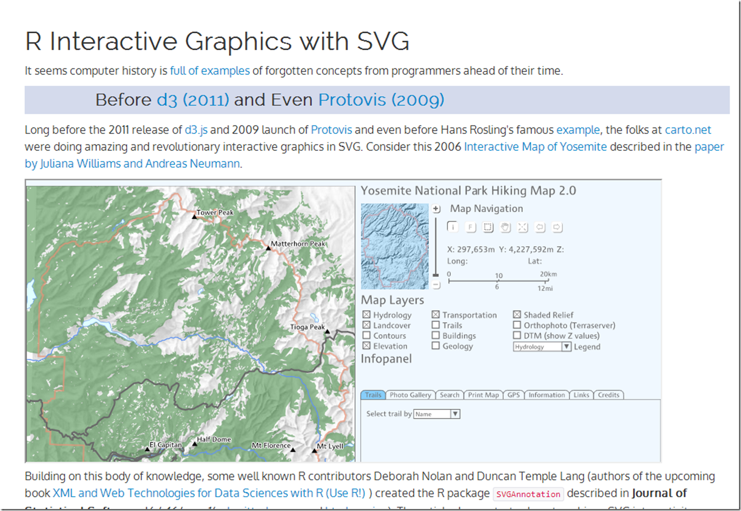
We R users are very spoiled by the ggplot2 and lattice engines that rival or beat the plotting libraries of any language.  Wouldn’t it be nice to have all the power of these engines to create interactive graphs?  Well, Paul Murrell, the author of grid (platform of ggplot2 and lattice), wrote gridSVG to do just that.  Over the last couple of years, Simon Potter under the guidance of Murrell has refined gridSVG for his honours project.  It is now a full-featured robust package capable of sending even your most complicated ggplot2 and lattice masterpieces to SVG.   gridSVG can do amazing things on his own, but I, of course, wanted to combine gridSVG with d3.  Click here or on the screenshot below to see a walkthrough applying a little gridSVG glue to ggplot2 and d3.

image

Thanks to Paul Murrell, Simon Potter, Hadley Wickham, Mike Bostock, Duncan Temple Lang, Deborah Nolan, Juliana Williams, Andreas Neumann, Ramnath Vaidyanathan and all the folks along the way that have made this possible.

Friday, June 28, 2013

rCharts Remake of NYT

For those wondering if I have forsaken finance, the answer is no.  I just don’t think there is much to do in here besides watch and wait.  So more d3 and R as I try to distract myself from doing something dumb in the markets.

This time I used rCharts and slidify to  recreate another NYT visualization similar to what I did in 512 Paths to the White House.  Now with any cumulative growth time series that we build in R we can apply the template and create this amazing visualization.  Below is a screenshot.  Click here to see the live version.

nyt home price rcharts

I’ll be living the good life over the next week, so no posts until after the 4th of July.

Thursday, June 27, 2013

dimple d3 and rCharts

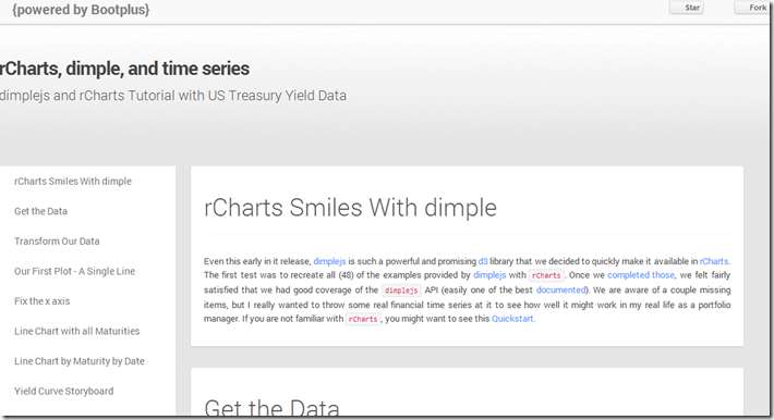
I put together a quick tutorial combining my two favorite things: finance and interactive visualizations.  I show how to use the new dimplejs d3 library with rCharts to create some nice interactive plots of US Treasury yield data.   A screenshot is below.  Go here for the tutorial and here for the code to reproduce.

image