REITs for Everybody Might Now Mean REITs for Nobody

THIS IS MY OPINION AND ANALYSIS AND IS NOT INVESTMENT ADVICE.  YOU ARE RESPONSIBLE FOR YOUR OWN GAINS AND LOSSES.

I think REITs traditionally attract conservative dividend investors (grandparents), but due to their recent behavior, REITs also attract beta chasers (hedge funds  and traders).  This additional demand has made REITs overvalued and even more volatile.  Both sets of REIT buyers might not want to buy now.

In terms of attractiveness to the traditional conservative dividend buyer, REITs seem unattractive on both an absolute and relative yield basis.

From TimelyPortfolio

From TimelyPortfolio

The newly found volatility of REITs for the beta chaser works well in a bullish stock market, but of course works in reverse on the downside.  This volatility also could easily scare the conservative long-term dividend buyer already concerned about low yields.

From TimelyPortfolio

From TimelyPortfolio

From TimelyPortfolio

From TimelyPortfolio

From TimelyPortfolio

One way to potentially dampen volatility would be to use a momentum type system as suggested by The Aleph Blog on REITs How to Make More Returns on REITs.  Results are pretty good.  Like the author, I was skeptical about his approach, since we would have no advance knowledge of momentum quintiles in 1971, but interestingly if we use the Dow Jones Industrial Average momentum quintiles 1896-1971, we would get very similar out of sample REIT results.

From TimelyPortfolio

From TimelyPortfolio

Please let me know what you think.

R code (click to download):

require(quantmod)
require(PerformanceAnalytics)   

#get NAREIT data
#I like NAREIT since I get back to 1971
#much easier though to get Wilshire REIT from FRED
#also it is daily instead of monthly
#getSymbols("WILLREITIND",src="FRED") will do this
require(gdata) 
reitURL <- "http://returns.reit.com/returns/MonthlyHistoricalReturns.xls"
reitExcel <- read.xls(reitURL,sheet="Data",pattern="All REITs",stringsAsFactors=FALSE)
#clean up dates so we can use xts functionality later
datetoformat <- reitExcel[,1]
datetoformat <- paste(substr(datetoformat,1,3),"-01-",substr(datetoformat,5,6),sep="")
datetoformat <- as.Date(datetoformat,format="%b-%d-%y")
reitExcel[,1] <- datetoformat     

#############now start the yield analysis#####################
#get REIT yield
reitYield <- as.xts(as.numeric(reitExcel[4:NROW(reitExcel),7]),
	order.by=reitExcel[4:NROW(reitExcel),1])
######get BAA and 10y from Fed to compare
getSymbols("BAA",src="FRED")
getSymbols("GS10",src="FRED")
######get SP500 yield from some multpl.com
##fantastic site with easily accessible historical information
spYield <- read.csv("http://www.multpl.com/s-p-500-dividend-yield/s-p-500-dividend-yield.csv")
spYield <- as.xts(spYield[,2],order.by=as.Date(spYield[,1]))
yieldCompare <- na.omit(merge(reitYield,spYield,BAA,GS10))
chart.TimeSeries(yieldCompare, legend.loc = "topleft",cex.legend=1.2,lwd=3,
	main="Yield Comparison of REITs with S&P500, BAA Yield, and US 10y Yield",
	colorset = c("cadetblue","darkolivegreen3","goldenrod","gray70"))
#get yield spread information
yieldSpread <- yieldCompare[,1:3]
yieldSpread[,1] <- yieldCompare[,1]-yieldCompare[,2]
yieldSpread[,2] <- yieldCompare[,1]-yieldCompare[,3]
yieldSpread[,3] <- yieldCompare[,1]-yieldCompare[,4]
colnames(yieldSpread) <- c("REIT Yield - S&P500 Yield",
	"REIT Yield - BAA Yield","REIT Yield - US 10y Yield")
chart.TimeSeries(yieldSpread, legend.loc = "topleft",cex.legend=1.2,lwd=3,
	main="Yield Spreads of REITs with S&P500, BAA Yield, and US 10y Yield",
	colorset = c("cadetblue","darkolivegreen3","goldenrod"))     

#############now start the return analysis###################
#shift colnames over 1
colnames(reitExcel) <- colnames(reitExcel)[c(1,1:(NCOL(reitExcel)-1))]
#get dates and return columns
reitData <- reitExcel[,c(3,24,38)]
#name columns
colnames(reitData) <- c(paste(colnames(reitExcel)[c(3,24,38)],".Total.Return",sep=""))
reitData <- reitData[3:NROW(reitData),]
#erase commas
col2cvt <- 1:NCOL(reitData)
reitData[,col2cvt] <- lapply(reitData[,col2cvt],function(x){as.numeric(gsub(",", "", x))}) 
#create xts
reitData <- as.xts(reitData,order.by=reitExcel[3:NROW(reitExcel),1])
#######get sp500 to compare beta and other measures
getSymbols("SP500",src="FRED")
SP500 <- to.monthly(SP500)[,4]
#get 1st of month to align when we merge
index(SP500) <- as.Date(index(SP500))
#merge REIT and S&p
returnCompare <- na.omit(merge(reitData,SP500))
returnCompare <- ROC(returnCompare,n=1,type="discrete")
charts.RollingRegression(returnCompare[, 1:3], returnCompare[,4],
	width=36,lwd = 3,legend.loc = "topleft",cex.legend=1.2,
	main="NAREIT REIT Indexes Compared to the S&P 500
	36 month Rolling",
	colorset=c("cadetblue","darkolivegreen3","goldenrod"))
chart.RollingPerformance(returnCompare,
	FUN="Return.annualized",width=36,lwd = 3,legend.loc = "topleft",cex.legend=1.2,
	main="NAREIT REIT Indexes Compared to the S&P 500
	36 month Rolling Return",
	colorset=c("cadetblue","darkolivegreen3","goldenrod","gray70"))
chart.RiskReturnScatter(returnCompare["1971::2003"],
	lwd = 3,legend.loc = "topleft",cex.legend=1.2,
	main="NAREIT REIT Indexes Compared to the S&P 500 1971-2003",
	colorset=c("cadetblue","darkolivegreen3","goldenrod","gray70"))
chart.RiskReturnScatter(returnCompare["2004::"],
	lwd = 3,legend.loc = "topleft",cex.legend=1.2,
	main="NAREIT REIT Indexes Compared to the S&P 500 Since 2004",
	colorset=c("cadetblue","darkolivegreen3","goldenrod","gray70"))
charts.PerformanceSummary(returnCompare,ylog=TRUE,
	lwd = 3,legend.loc = "topleft",cex.legend=1.2,
	main="NAREIT REIT Indexes Compared to the S&P 500",
	colorset=c("cadetblue","darkolivegreen3","goldenrod","gray70"))         

#############now start the bucket analysis###################
#bucket momentum as described by Aleph Blog
#get 10 month moving average
#set up avg with same as reitData
avg <- reitData[,1:3]
avg <- as.data.frame(avg)
avg[,1:3] <- lapply(reitData[,1:3],runMean,n=10)
avg <- as.xts(avg)
#get % above 10 month moving average
momscore <- reitData/avg-1
#break into 5 evenly distributed by frequency quintiles
#get signal into 3 column xts
signal <- momscore
for(i in 1:3) {
	breaks <- quantile(momscore[,i], probs = seq(0, 1, 0.20),na.rm=TRUE)
	#use default labels=TRUE to see how this works
	buckets <- cut(momscore[,i], include.lowest=TRUE, breaks=breaks)
	#store so we can see later
	ifelse(i==1,bucket_ranges <- names(table(buckets)),
		bucket_ranges <- rbind(bucket_ranges,names(table(buckets))))
	#now use labels=FALSE to return 1-5 based on quintile
	buckets <- cut(momscore[,i], breaks=breaks, labels=FALSE)
	signal[,i] <- as.xts(buckets,order.by=index(signal))
	#move forward by 1
}
#name bucket_ranges with reit column names
rownames(bucket_ranges)<-colnames(reitData)
signal <- lag(signal,k=1)
ret <- signal
#showing my R weakness here and had to go back to for..next
for(i in 1:3) {
	ret[,i] <- ifelse(signal[,i] >= 3,1,0) * ROC(reitData[,1],1,type="discrete")
}
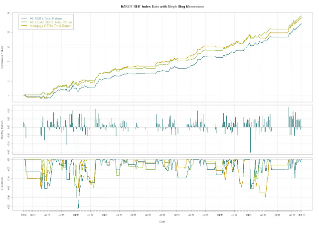
charts.PerformanceSummary(ret,ylog=TRUE,legend.loc = "topleft",cex.legend=1.2,
	main="NAREIT REIT Index Data with Aleph Blog Momentum",
	colorset=c("cadetblue","darkolivegreen3","goldenrod"))     

getSymbols("DJIA",src="FRED")
#examine DJIA quantiles prior to 1973 to see if we could
#know in advance what possible REIT quantiles would work
DJIA <- to.monthly(DJIA)["1896::1971",4]
momDJIA <- DJIA/runMean(DJIA,n=10)-1
breaks <- quantile(momDJIA, probs = seq(0, 1, 0.20),na.rm=TRUE)
buckets <- cut(momDJIA, breaks=breaks)
table(buckets)   

#what happens if we apply the DJIA prior to 1973 buckets to the REITs
ret <- merge(ret,ret)
for(i in 1:3) {
	#if REITs > 3.95% above 10 month moving average then long
	#3.95% is the lower end of the DJIA 1896-1971 3 momentum quantile
	ret[,i+3] <- lag(ifelse(momscore[,i] >= 0.0395,1,0),1) * ROC(reitData[,1],1,type="discrete")
}
colnames(ret)[4:6]<-paste(colnames(reitData[,1:3])," with DJIA buckets",sep="")
#much much better than I expected
charts.PerformanceSummary(ret,ylog=TRUE,legend.loc = "topleft",cex.legend=1.2,
	main="NAREIT REIT Index Data with Aleph Blog Momentum but DJIA Momentum Buckets",
	colorset=c("cadetblue","darkolivegreen3","goldenrod",
	"coral","darkorchid","darkolivegreen"))

Created by Pretty R at inside-R.org