Happy Thanksgiving | More Examples of XML + rvest with SVG

I did not intend for this little experiment to become a post, but I think the code builds nicely on the XML + rvest combination (also see yesterday’s post) for working with XML/HTML/SVG documents in R.

It all started when I was playing on my iPhone in the Sketchbook app and drew a really bad turkey.  Even though, the turkey was bad, I thought it would be fun to combine with vivus.js.  However, Sketchbook does not export SVG, so I exported as PDF and imported into Inkscape.  The end result was a still very messy SVG file, so I thought it would be a great test / application of my new skills with rvest + XML. The code opens the SVG, grabs all the path nodes, assembles those into a svg tag with id = "turkey", and then adds a script to use the addDependency for vivus.js.

Happy Thanksgiving to all the US readers out there.

Slightly Advanced rvest with Help from htmltools + XML + pipeR

Hadley Wickham’s post “rvest: easy web scraping with R” introduces the fine new package rvest very well.  For those now yearning a slightly more advanced example with a little help from pipeR + htmltools + XML, I thought this might fill your yearn.  The code grabs css information running the fancy new site cssstats.com on my blog site.  With the background colors, it makes and labels some swatches and outputs them to the RStudio viewer--if installed--or your browser if not.

library(pipeR)
library(htmltools)
library(rvest)
library(XML)

# some slightly more advanced exercises
# using rvest, XML, and htmltools

# this one takes all the svg nodes in the section
# with id unique-background-colors from the 
# site cssstats.com run on timelyportfolio.blogspot.com
# 1) removes attributes
# 2) sizes them at 85px x 64px
# 3) add new text node with fill value
# 4) combines them into a single div
# 5) with some meta information
"http://cssstats.com/stats?url=http%3A%2F%2Ftimelyportfolio.blogspot.com" %>>%
  html %>>%
  html_nodes( "#unique-background-colors svg" ) %>>%
  xmlApply( function(x){
    removeAttributes(x)
    addAttributes(x,style="display:inline-block;height:85px;width:64px")
    fillNode = newXMLNode(
      "text"
      ,html_attr(html_node(x,"rect"),"fill")
      ,attrs=c(x=0,y=75,style="font-size:70%")
    )
    addChildren(x,fillNode)
    saveXML(x) %>>% HTML
  } ) %>>%
  (tags$div(
    style="display:inline-block;height:100%;width:100%"
    ,list(
      tags$h3(
        "Colors of TimelyPortfolio from "
        ,tags$a(href="http://cssstats.com","cssstats")
      )
      ,.
    )
  )) %>>%
  tagList %>>%
  html_print

I just copied the div output below in Windows Live Writer (notably from JJ Allaire and Joe Cheng of RStudio).

Colors of TimelyPortfolio from cssstats

Secret to Making Things Appear in RStudio Viewer

I am by no means an authoritative source on this, but I think I found out the secret behind htmltools html_print that chooses the RStudio Viewer browser rather than your default browser like utils::browseURL. Here is a quick code snippet that hopefully explains what is happening. It appears you just need a temp directory with the pattern starting with viewhtml*.

library(htmltools)
library(pipeR)

# htmltools from RStudio very nicely
# makes things appear in the Viewer Window
"<h3>Hello in RStudio Viewer</h3>" %>>%
  HTML %>>%
  html_print


# there is a little secret to doing the same
# without htmltools
"<h3>Hello in RStudio Viewer</h3>" %>>%
  HTML %>>%
  # and the secret is to place in a temp directory
  # with the pattern viewhtml
  (
  ht ~
    tempfile("viewhtml") %>>%
    (~ dir.create(.) ) %>>%
    (~ save_html(ht, file = file.path(.,"index.html")) ) %>>%
    ( getOption("viewer")(file.path(.,"index.html")) )
  )
  
# to see it in action look at the code change
# in this project
utils::browseURL("https://github.com/bryanhanson/exCon/pull/1/files")

The only reason I mention it is that I much prefer to stay in the RStudio environment instead of switching contexts to a browser.  I still firmly recommend using tags from htmltools as the best method to make all this work seamlessly and as intended by the experts at RStudio. 

Pipeline to Plot Annual % Change

(thanks tradeblotter for pointing out error in code in first release)

Pipes in R make my life incredibly easy, and I think my code easier to read.   Note, there are a couple different flavors of pipes (see magrittr and pipeR).  For now, I choose pipeR.

library(quantmod)
library(pipeR)
library(ggplot2)

getSymbols("^GSPC",from="1900-01-01",auto.assign=F) %>>% #get S&P 500 from Yahoo!Finance
  ( .[endpoints(.,"years"),4] ) %>>% #get end of year
  ROC( type="discrete", n=1 ) %>>%   #get one year rate of change
  na.fill(0) %>>%                    #fill first year with 0
  (                                  #make data.frame
    data.frame(
      date = as.Date(format(index(.),"%Y-01-01"))
      ,.
    )
  ) %>>%
  structure(                         #hard way to do colnames()
    names = c("date","change")
  ) %>>%
  ggplot(                            #start our plot pipe
    aes( y= change, x=  date)
  ) %>>%
  + geom_bar( stat="identity" ) %>>% #choose bar
  + labs( title = "Annual Change of the S&P 500" ) #give plot a title

Or if we wanted to use the new pipeline syntax for the plot portion.

library(quantmod)
library(pipeR)
library(ggplot2)

getSymbols("^GSPC",from="1900-01-01",auto.assign=F) %>>% #get S&P 500 from Yahoo!Finance
  ( .[endpoints(.,"years"),4] ) %>>% #get end of year
  ROC( type="discrete", n=1 ) %>>%   #get one year rate of change
  na.fill(0) %>>%                    #fill first year with 0
  (                                  #make data.frame
    data.frame(
      date = as.Date(format(index(.),"%Y-01-01"))
      ,.
    )
  ) %>>%
  structure(                         #hard way to do colnames()
    names = c("date","change")
  ) %>>%
  (
    pipeline({
      ggplot(., aes( y= change, x=  date) )
      + geom_bar( stat="identity" )
      + labs( title = "Annual Change of the S&P 500 (source: Yahoo! Finance)" )
    })
  )

Update on JGBs versus USTs

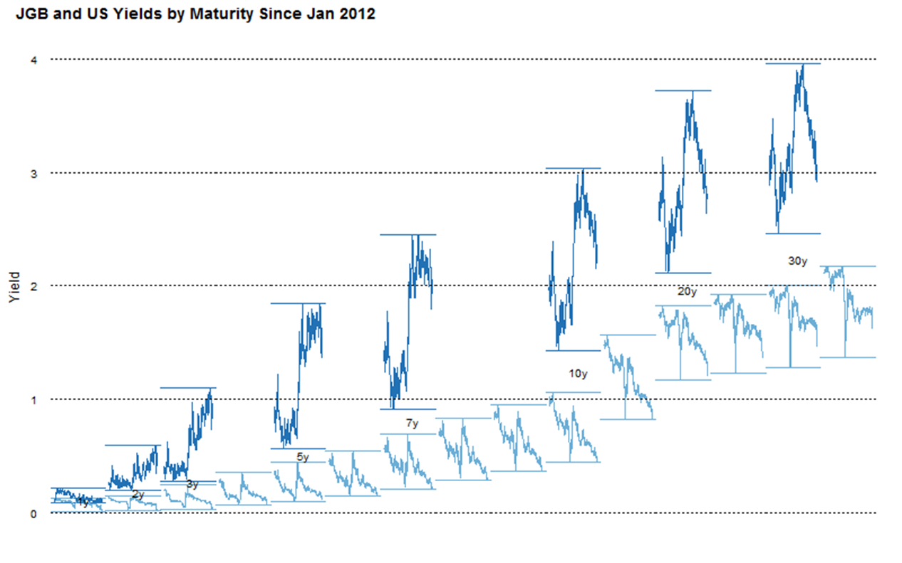
Given the recent selloff in the Yen, I thought now would be a good time to update my favorite chart from Intended or Unintended Consequences.

For a true currency death spiral, rates need to move up rather than down.  It appears we are long way from that.

Long-time readers will know that I have been keenly interested in the Yen for the entire history of this blog http://timelyportfolio.blogspot.com/search?q=yen.

Code for this post: https://gist.github.com/timelyportfolio/5665790