THIS IS NOT INVESTMENT ADVICE. YOU ARE RESPONSIBLE FOR YOUR OWN GAINS AND LOSSES.
I did not intend for this to be a two-part series but I just could not be complacent with Utility Spread and Financial Turbulence (for avid readers, there was a small error in this post that is now corrected). Since the change was so easy and the results so much better, I thought I should share.
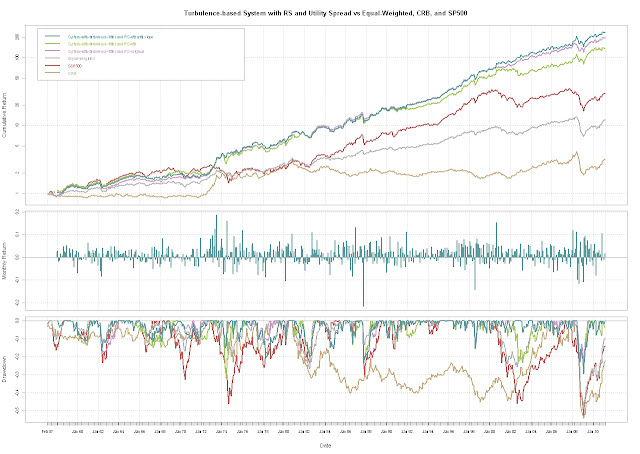
In previous posts, I set up a very basic relative strength approach by using the 12 month slope (linear beta) to choose the stronger performer. The improvements from adding this relative strength technique to my original Great FAJ Article on Statistical Measure of Financial Turbulence system were substantial as seen in Great FAJ Article on Statistical Measure of Financial Turbulence Part 3. If the technique has helped in the past and I already know how to do the calculation, I figured I should at least try to apply it to the Utility Spread. Now when turbulence is low, invest in the stronger of the S&P 500 and CRB, but when turbulence is high, use the Utility Spread only if its 12 month slope is positive. If everything is blowing up (turbulence high) and utilities are not defensive (slope is negative), then use the US 10y Treasury as your last resort. Lots of rules but they intuitively make sense to me. Drawdown remains higher than I would like.
 |
| From TimelyPortfolio |
R code (thanks patrick for the comment to make code more readable):
#cleaned up the code to eliminate leftovers from previous posts and studies
#see http://timelyportfolio.blogspot.com for the history and older code   require(quantmod)
require(PerformanceAnalytics)   #get data from St. Louis Federal Reserve (FRED)
getSymbols("GS20",src="FRED") #load 20yTreasury; 20y has gap 86-93; 30y has gap in early 2000s
getSymbols("GS30",src="FRED") #load 30yTreasury to fill 20y gap 86-93
getSymbols("GS10",src="FRED") #load 10yTreasury
getSymbols("BAA",src="FRED") #load BAA
getSymbols("SP500",src="FRED") #load SP500
#now Dow Jones Indexes
getSymbols("DJIA",src="FRED") #load daily Dow Jones Industrial
getSymbols("DJUA",src="FRED") #load daily Dow Jones Utility   DJUADJIA <- DJUA/DJIA   #get CRB data from a csv file
CRB <- as.xts(read.csv("crb.csv",row.names=1))[,1]   #fill 20y gap from discontinued 20y Treasuries with 30y
GS20["1987-01::1993-09"] <- GS30["1987-01::1993-09"]   #do a little manipulation to get the data lined up on monthly basis
SP500  <-  to.monthly(SP500)[,4]
GS10  <-  to.monthly(GS10)[,4]
DJUADJIA <- to.monthly(DJUADJIA)[,4]
#get monthly format to yyyy-mm-dd with the first day of the month
index(SP500) <- as.Date(index(SP500))
index(GS10) <- as.Date(index(GS10))
index(DJUADJIA) <- as.Date(index(DJUADJIA))
#my CRB data is end of month; could change but more fun to do in R
CRB <- to.monthly(CRB)[,4]
index(CRB) <- as.Date(index(CRB))   #let's merge all this into one xts object; CRB starts last in 1956
assets <- na.omit(merge(GS20,SP500,CRB,DJUADJIA))
#use ROC for SP500 and CRB and momentum for yield data
assetROC <- na.omit(merge(momentum(assets[,1])/100,ROC(assets[,2:4],type="discrete")))   ############Turbulence calculation
#get Correlations
corrBondsSp <- runCor(assetROC[,1],assetROC[,2],n=7)
corrBondsCrb <- runCor(assetROC[,1],assetROC[,3],n=7)
corrSpCrb <- runCor(assetROC[,2],assetROC[,3],n=7)
#composite measure of correlations between asset classes and roc-weighted correlations
assetCorr <- (corrBondsSp+corrBondsCrb+corrSpCrb+
	(corrBondsSp*corrSpCrb*assetROC[,2])+
	(corrBondsCrb*corrSpCrb*assetROC[,3])-
	assetROC[,1])/6
#sum of ROCs of asset classes
assetROCSum <- assetROC[,1]+assetROC[,2]+assetROC[,3]
#finally the turbulence measure
turbulence <- abs(assetCorr*assetROCSum*100)
colnames(turbulence) <- "Turbulence-correlation"
############   ############Get Bond Return Data
#get bond returns to avoid proprietary data problems
#see previous timelyportfolio blogposts for explanation
#probably need to make this a function since I will be using so much
require(RQuantLib)
GS10pricereturn <- GS10  #set this up to hold price returns   GS10pricereturn[1,1] <- 0
colnames(GS10pricereturn) <- "BondPriceReturn"
#I know I need to vectorize this but not qualified enough yet
#Please feel free to comment to show me how to do this
for (i in 1:(NROW(GS10)-1)) {
  GS10pricereturn[i+1,1] <- FixedRateBondPriceByYield(yield=GS10[i+1,1]/100,issueDate=Sys.Date(),
	maturityDate= advance("UnitedStates/GovernmentBond", Sys.Date(), 10, 3),
	rates=GS10[i,1]/100,period=2)[1]/100-1
}   #interest return will be yield/12 for one month
GS10interestreturn <- lag(GS10,k=1)/12/100
colnames(GS10interestreturn) <- "BondInterestReturn"   #total return will be the price return + interest return
GS10totalreturn <- GS10pricereturn + GS10interestreturn
colnames(GS10totalreturn) <- "BondTotalReturn"
assetROC <- na.omit(merge(GS10totalreturn,ROC(assets[,2:4],type="discrete")))
############   ############System building
#wish I could remember where I got some of this code
#most likely candidate is www.fosstrading.com
#please let me know if you know the source
#so I can give adequate credit   #let's use basic relative strength to pick sp500 or crb
#know I can do this better in R but here is my ugly code
#to calculate 12 month slope of sp500/crb and djua/djia
width=12
for (i in 1:(NROW(assets)-width)) {
	#get sp500/crb slope
	model <- lm(assets[i:(i+width),2]/assets[i:(i+width),3]~index(assets[i:(i+width)]))
	ifelse(i==1,assetSlope <- model$coefficients[2],assetSlope <- rbind(assetSlope,model$coefficients[2]))
	#get djua/djia slope; already calculated ratio so just take that
	model_util <- lm(assets[i:(i+width),4]~index(assets[i:(i+width)]))
	ifelse(i==1,assetSlopeUtil <- model_util$coefficients[2],assetSlopeUtil <- rbind(assetSlopeUtil,model_util$coefficients[2]))
}
assetSlope <- xts(cbind(assetSlope),order.by=index(assets)[(width+1):NROW(assets)])
assetSlopeUtil <- xts(cbind(assetSlopeUtil),order.by=index(assets)[(width+1):NROW(assets)])
assetSlope <- merge(assetSlope,assetSlopeUtil)
#use turbulence to determine in or out of equal-weighted sp500 and crb
signal <- ifelse(turbulence>0.8,0,1)   #use slope of sp500/crb to determine sp500 or crb
signal2 <- ifelse(assetSlope[,1]>0,1,2)   #lag signals
#if we knew what would happen tomorrow, we can eliminate all this effort
signal <- lag(signal,k=1)
signal[1] <- 0
signal2 <- lag(signal2,k=1)
signal2[1] <- 0   signals_returns <- merge(signal,signal2,assetROC,assetSlope)
#get sp500 or crb return based on slope when turbulence low or use bonds as cash
ret <- ifelse(signals_returns[,2]==1&signals_returns[,1]==1,signals_returns[,4],
	ifelse(signals_returns[,2]==2&signals_returns[,1]==1,signals_returns[,5],
	signals_returns[,3]))
#get sp500 or crb return based on slope when turbulence low or use utility spread as cash
ret_util <- ifelse(signals_returns[,2]==1&signals_returns[,1]==1,signals_returns[,4],
	ifelse(signals_returns[,2]==2&signals_returns[,1]==1,signals_returns[,5],
	signals_returns[,6]))
#get sp500 or crb return based on slope when turbulence low or use utility spread
#as cash only if slope positive
ret_util_slope <- ifelse(signals_returns[,2]==1&signals_returns[,1]==1,signals_returns[,4],
	ifelse(signals_returns[,2]==2&signals_returns[,1]==1,signals_returns[,5],
	ifelse(signals_returns[,8]>0,signals_returns[,6],signals_returns[,3])))
ret_util[1] <- 0
ret_util_slope[1] <- 0   #get system performance
system_perf_rs <- ret
system_perf_rs_util <- ret_util
system_perf_rs_util_slope <- ret_util_slope   perf_comparison <- merge(system_perf_rs_util_slope,system_perf_rs_util,system_perf_rs,(assetROC[,2]+assetROC[,3])/2,assetROC[,2],assetROC[,3])
colnames(perf_comparison) <- c("System-with-turbulence-filter and RS-util with slope",
	"System-with-turbulence-filter and RS-util", "System-with-turbulence-filter and RS-original",
	"Equal-weighted","S&P500","CRB")   charts.PerformanceSummary(perf_comparison,ylog=TRUE,
	main="Turbulence-based System with RS and Utility Spread vs Equal-Weighted, CRB, and SP500",
	colorset=c("cadetblue","darkolivegreen3","plum3","gray70","indianred","burlywood3"))
I thought about a similar technique on my commute today and wondered if it would make any difference. Thanks for the research and part2!!
ReplyDeleteYour R code would be easier to read if you used more spaces. Especially useful for comprehension is spaces around the assignment operator. Important for getting it right is spaces around comparison operators -- see 'The R Inferno' http://www.burns-stat.com/pages/Tutor/R_inferno.pdf page 62.
ReplyDelete