Wednesday, May 25, 2011

Eigen-who? How Can I Write About Eigen-anything and Expect You to Read?

After the very nice Convore reply

@timelyportfolio some of your posts include "eigenvalue ratio plots" -- kindly tell us what they show and how they might be useful in constructing a portfolio.

I felt like I should at least attempt to offer a little more detail on eigenvectors, which allow us to visually see similarity between variables (in my mind, time series of asset classes, indexes, stocks, or other financial prices).  In other posts, I have used the fAssets package function assetsCorEigenPlot for Long XLU Short SPY and  Russell Napier, ASIP in FT Says Emerging Market CurrenciesMichael Friendly’s wonderful paper does a very fine job of explaining eigenvalues and their use in sorting for helpful visualizations of correlation.  Wikipedia also gives a decent introduction in these two articles http://en.wikipedia.org/wiki/Principal_component_analysis and http://en.wikipedia.org/wiki/Eigenvector.  Also, I’m anxious to read the following book whose authors run http://factominer.free.fr/classical-methods/index.html

Really, the closer the variables in distance and angle, the more closely they are related.  I thought some currency data from the St. Louis Fed would provide a nice example.  Similar to milktrader’s Chop, Slice and Dice Your Returns in R, I also wanted to show multiple ways in R of achieving a plot of eigenvalues with fAssets, SciViews, and corrgram.  This analysis does not yield any real surprises—Mexican Peso and Brazilian Real are closely related, but both are least related to the Japanese Yen.

From TimelyPortfolio

Since I used Michael Friendly’s paper so much in writing this article, I wanted to show a corrgram of the currency data.  The corrgram package offers lots of potentially useful variations of this visualization.

From TimelyPortfolio

The second part of the Convore question is how can we use eigenvalues to construct a portfolio.  Maybe I can answer that in one of my next posts…

R code:

#explain basics of principal component analysis
#by showing the various methods of charting eigenvalues
#of currency data   #give specific credit to Michael Friendly
#and his paper http://www.math.yorku.ca/SCS/Papers/corrgram.pdf
#another example of similar techniques used for both
#baseball and finance   #for additional information on principal component analysis (PCA)
#see http://en.wikipedia.org/wiki/Principal_component_analysis   require(quantmod)   #get currency data from the FED FRED data series
Korea <- getSymbols("DEXKOUS",src="FRED",auto.assign=FALSE) #load Korea
Malaysia <- getSymbols("DEXMAUS",src="FRED",auto.assign=FALSE) #load Malaysia
Singapore <- getSymbols("DEXSIUS",src="FRED",auto.assign=FALSE) #load Singapore
Taiwan <- getSymbols("DEXTAUS",src="FRED",auto.assign=FALSE) #load Taiwan
China <- getSymbols("DEXCHUS",src="FRED",auto.assign=FALSE) #load China
Japan <- getSymbols("DEXJPUS",src="FRED",auto.assign=FALSE) #load Japan
Thailand <- getSymbols("DEXTHUS",src="FRED",auto.assign=FALSE) #load Thailand
Brazil <- getSymbols("DEXBZUS",src="FRED",auto.assign=FALSE) #load Brazil
Mexico <- getSymbols("DEXMXUS",src="FRED",auto.assign=FALSE) #load Mexico
India <- getSymbols("DEXINUS",src="FRED",auto.assign=FALSE) #load India
USDOther <- getSymbols("DTWEXO",src="FRED",auto.assign=FALSE) #load US Dollar Other Trading Partners
USDBroad <- getSymbols("DTWEXB",src="FRED",auto.assign=FALSE) #load US Dollar Broad   #combine all the currencies into one big currency xts
currencies<-merge(Korea, Malaysia, Singapore, Taiwan,
China, Japan, Thailand, Brazil, Mexico, India,
USDOther, USDBroad)
currencies<-na.omit(currencies)
colnames(currencies)<-c("Korea", "Malaysia", "Singapore", "Taiwan",
"China", "Japan", "Thailand", "Brazil", "Mexico", "India",
"USDOther", "USDBroad")
#get daily percent changes
currencies<-currencies/lag(currencies)-1       #using fAssets
require(fAssets)
assetsCorEigenPlot(as.timeSeries(currencies))       #using techniques from corrgram package documentation
#get correlation matrix
(currencies.cor <- cor(currencies,use="pair"))
#get two largest eigenvectors
(currencies.eig<-eigen(currencies.cor)$vectors[,1:2])
e1 <- currencies.eig[,1]
e2 <- currencies.eig[,2]
#make the chart
plot(e1,e2,col='white', xlim=range(e1,e2), ylim=range(e1,e2),
main="Plot of 2 Largest Eigenvectors for Various Asian
and American Currencies (corrgram)"
)
arrows(0, 0, e1, e2, cex=0.5, col="red", length=0.1)
text(e1,e2, rownames(currencies.cor), cex=0.75)
#run an interesting corrgram chart
require(corrgram) #do not need for previous eigenvector plot
df1 <- data.frame(cbind(index(currencies),coredata(currencies)))
corrgram(df1, order=TRUE,
main="Currency data PC2/PC1 order",
lower.panel=panel.shade, upper.panel=panel.pie,
text.panel=panel.txt)       #using techniques from SciViews package
#do principal component analysis
require(SciViews)
(currencies.pca <- pcomp(~Korea + Malaysia + Singapore + Taiwan +
China + Japan + Thailand + Brazil + Mexico + India +
USDOther + USDBroad,
data = currencies))
#make the chart
plot(currencies.pca, which = "correlations",
main="Plot of 2 Largest Eigenvectors for Various Asian
and American Currencies (SciViews)"
)
#more SciViews fun
#summary(currencies.pca)
#screeplot(currencies.pca)
#currencies.ldg<-loadings(currencies.pca)
#(currencies.cor <- correlation(currencies.pca))
#plot(currencies.pca, which = "scores", cex = 0.8)
#pairs(currencies.pca)         #compare 2 largest eigenvectors from the sciview and corrgram
cbind(loadings(currencies.pca)[,1],e1,loadings(currencies.pca)[,2],e2)
Created by Pretty R at inside-R.org

Tuesday, May 24, 2011

Utility Spread and Financial Turbulence Part 2 with Utility Slope

THIS IS NOT INVESTMENT ADVICE.  YOU ARE RESPONSIBLE FOR YOUR OWN GAINS AND LOSSES.

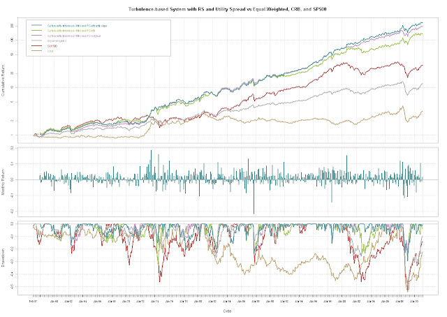
I did not intend for this to be a two-part series but I just could not be complacent with Utility Spread and Financial Turbulence (for avid readers, there was a small error in this post that is now corrected).  Since the change was so easy and the results so much better, I thought I should share.

In previous posts, I set up a very basic relative strength approach by using the 12 month slope (linear beta) to choose the stronger performer.  The improvements from adding this relative strength technique to my original Great FAJ Article on Statistical Measure of Financial Turbulence system were substantial as seen in Great FAJ Article on Statistical Measure of Financial Turbulence Part 3.  If the technique has helped in the past and I already know how to do the calculation, I figured I should at least try to apply it to the Utility Spread.  Now when turbulence is low, invest in the stronger of the S&P 500 and CRB, but when turbulence is high, use the Utility Spread only if its 12 month slope is positive.  If everything is blowing up (turbulence high) and utilities are not defensive (slope is negative), then use the US 10y Treasury as your last resort.  Lots of rules but they intuitively make sense to me.  Drawdown remains higher than I would like.

From TimelyPortfolio

R code (thanks patrick for the comment to make code more readable):

#cleaned up the code to eliminate leftovers from previous posts and studies
#see http://timelyportfolio.blogspot.com for the history and older code   require(quantmod)
require(PerformanceAnalytics)   #get data from St. Louis Federal Reserve (FRED)
getSymbols("GS20",src="FRED") #load 20yTreasury; 20y has gap 86-93; 30y has gap in early 2000s
getSymbols("GS30",src="FRED") #load 30yTreasury to fill 20y gap 86-93
getSymbols("GS10",src="FRED") #load 10yTreasury
getSymbols("BAA",src="FRED") #load BAA
getSymbols("SP500",src="FRED") #load SP500
#now Dow Jones Indexes
getSymbols("DJIA",src="FRED") #load daily Dow Jones Industrial
getSymbols("DJUA",src="FRED") #load daily Dow Jones Utility   DJUADJIA <- DJUA/DJIA   #get CRB data from a csv file
CRB <- as.xts(read.csv("crb.csv",row.names=1))[,1]   #fill 20y gap from discontinued 20y Treasuries with 30y
GS20["1987-01::1993-09"] <- GS30["1987-01::1993-09"]   #do a little manipulation to get the data lined up on monthly basis
SP500 <- to.monthly(SP500)[,4]
GS10 <- to.monthly(GS10)[,4]
DJUADJIA <- to.monthly(DJUADJIA)[,4]
#get monthly format to yyyy-mm-dd with the first day of the month
index(SP500) <- as.Date(index(SP500))
index(GS10) <- as.Date(index(GS10))
index(DJUADJIA) <- as.Date(index(DJUADJIA))
#my CRB data is end of month; could change but more fun to do in R
CRB <- to.monthly(CRB)[,4]
index(CRB) <- as.Date(index(CRB))   #let's merge all this into one xts object; CRB starts last in 1956
assets <- na.omit(merge(GS20,SP500,CRB,DJUADJIA))
#use ROC for SP500 and CRB and momentum for yield data
assetROC <- na.omit(merge(momentum(assets[,1])/100,ROC(assets[,2:4],type="discrete")))   ############Turbulence calculation
#get Correlations
corrBondsSp <- runCor(assetROC[,1],assetROC[,2],n=7)
corrBondsCrb <- runCor(assetROC[,1],assetROC[,3],n=7)
corrSpCrb <- runCor(assetROC[,2],assetROC[,3],n=7)
#composite measure of correlations between asset classes and roc-weighted correlations
assetCorr <- (corrBondsSp+corrBondsCrb+corrSpCrb+
(corrBondsSp*corrSpCrb*assetROC[,2])+
(corrBondsCrb*corrSpCrb*assetROC[,3])-
assetROC[,1])/6
#sum of ROCs of asset classes
assetROCSum <- assetROC[,1]+assetROC[,2]+assetROC[,3]
#finally the turbulence measure
turbulence <- abs(assetCorr*assetROCSum*100)
colnames(turbulence) <- "Turbulence-correlation"
############   ############Get Bond Return Data
#get bond returns to avoid proprietary data problems
#see previous timelyportfolio blogposts for explanation
#probably need to make this a function since I will be using so much
require(RQuantLib)
GS10pricereturn <- GS10 #set this up to hold price returns   GS10pricereturn[1,1] <- 0
colnames(GS10pricereturn) <- "BondPriceReturn"
#I know I need to vectorize this but not qualified enough yet
#Please feel free to comment to show me how to do this
for (i in 1:(NROW(GS10)-1)) {
GS10pricereturn[i+1,1] <- FixedRateBondPriceByYield(yield=GS10[i+1,1]/100,issueDate=Sys.Date(),
maturityDate= advance("UnitedStates/GovernmentBond", Sys.Date(), 10, 3),
rates=GS10[i,1]/100,period=2)[1]/100-1
}   #interest return will be yield/12 for one month
GS10interestreturn <- lag(GS10,k=1)/12/100
colnames(GS10interestreturn) <- "BondInterestReturn"   #total return will be the price return + interest return
GS10totalreturn <- GS10pricereturn + GS10interestreturn
colnames(GS10totalreturn) <- "BondTotalReturn"
assetROC <- na.omit(merge(GS10totalreturn,ROC(assets[,2:4],type="discrete")))
############   ############System building
#wish I could remember where I got some of this code
#most likely candidate is www.fosstrading.com
#please let me know if you know the source
#so I can give adequate credit   #let's use basic relative strength to pick sp500 or crb
#know I can do this better in R but here is my ugly code
#to calculate 12 month slope of sp500/crb and djua/djia
width=12
for (i in 1:(NROW(assets)-width)) {
#get sp500/crb slope
model <- lm(assets[i:(i+width),2]/assets[i:(i+width),3]~index(assets[i:(i+width)]))
ifelse(i==1,assetSlope <- model$coefficients[2],assetSlope <- rbind(assetSlope,model$coefficients[2]))
#get djua/djia slope; already calculated ratio so just take that
model_util <- lm(assets[i:(i+width),4]~index(assets[i:(i+width)]))
ifelse(i==1,assetSlopeUtil <- model_util$coefficients[2],assetSlopeUtil <- rbind(assetSlopeUtil,model_util$coefficients[2]))
}
assetSlope <- xts(cbind(assetSlope),order.by=index(assets)[(width+1):NROW(assets)])
assetSlopeUtil <- xts(cbind(assetSlopeUtil),order.by=index(assets)[(width+1):NROW(assets)])
assetSlope <- merge(assetSlope,assetSlopeUtil)
#use turbulence to determine in or out of equal-weighted sp500 and crb
signal <- ifelse(turbulence>0.8,0,1)   #use slope of sp500/crb to determine sp500 or crb
signal2 <- ifelse(assetSlope[,1]>0,1,2)   #lag signals
#if we knew what would happen tomorrow, we can eliminate all this effort
signal <- lag(signal,k=1)
signal[1] <- 0
signal2 <- lag(signal2,k=1)
signal2[1] <- 0   signals_returns <- merge(signal,signal2,assetROC,assetSlope)
#get sp500 or crb return based on slope when turbulence low or use bonds as cash
ret <- ifelse(signals_returns[,2]==1&signals_returns[,1]==1,signals_returns[,4],
ifelse(signals_returns[,2]==2&signals_returns[,1]==1,signals_returns[,5],
signals_returns[,3]))
#get sp500 or crb return based on slope when turbulence low or use utility spread as cash
ret_util <- ifelse(signals_returns[,2]==1&signals_returns[,1]==1,signals_returns[,4],
ifelse(signals_returns[,2]==2&signals_returns[,1]==1,signals_returns[,5],
signals_returns[,6]))
#get sp500 or crb return based on slope when turbulence low or use utility spread
#as cash only if slope positive
ret_util_slope <- ifelse(signals_returns[,2]==1&signals_returns[,1]==1,signals_returns[,4],
ifelse(signals_returns[,2]==2&signals_returns[,1]==1,signals_returns[,5],
ifelse(signals_returns[,8]>0,signals_returns[,6],signals_returns[,3])))
ret_util[1] <- 0
ret_util_slope[1] <- 0   #get system performance
system_perf_rs <- ret
system_perf_rs_util <- ret_util
system_perf_rs_util_slope <- ret_util_slope   perf_comparison <- merge(system_perf_rs_util_slope,system_perf_rs_util,system_perf_rs,(assetROC[,2]+assetROC[,3])/2,assetROC[,2],assetROC[,3])
colnames(perf_comparison) <- c("System-with-turbulence-filter and RS-util with slope",
"System-with-turbulence-filter and RS-util", "System-with-turbulence-filter and RS-original",
"Equal-weighted","S&P500","CRB")   charts.PerformanceSummary(perf_comparison,ylog=TRUE,
main="Turbulence-based System with RS and Utility Spread vs Equal-Weighted, CRB, and SP500",
colorset=c("cadetblue","darkolivegreen3","plum3","gray70","indianred","burlywood3"))

Created by Pretty R at inside-R.org

Monday, May 23, 2011

Utility Spread and Financial Turbulence

THIS IS NOT INVESTMENT ADVICE.  YOU ARE RESPONSIBLE FOR YOUR OWN GAINS AND LOSSES.

In Long XLU Short SPY Part 2 (More History), I explored the defensive nature of the spread and its potential as a bond substitute in troublesome periods for stocks.  I thought it would be interesting to see what happens if we use the spread as our cash position in the Great FAJ Article on Statistical Measure of Financial Turbulence Part 3 system.  Unfortunately, the use of the spread on price returns as cash does not benefit the system as much as bonds as cash, but I still thought it might encourage some additional reader thought on the spread and its potential uses.

From TimelyPortfolio

R code:

require(quantmod)
require(PerformanceAnalytics)

#get data from St. Louis Federal Reserve (FRED)
getSymbols("GS20",src="FRED") #load 20yTreasury; 20y has gap 86-93; 30y has gap in early 2000s
getSymbols("GS30",src="FRED") #load 30yTreasury to fill 20y gap 86-93
getSymbols("BAA",src="FRED") #load BAA
getSymbols("SP500",src="FRED") #load SP500
#now Dow Jones Indexes
getSymbols("DJIA",src="FRED") #load daily Dow Jones Industrial
getSymbols("DJUA",src="FRED") #load daily Dow Jones Utility

DJUADJIA<-DJUA/DJIA

#get CRB data from a csv file
CRB<-as.xts(read.csv("crb.csv",row.names=1))[,1]

#fill 20y gap from discontinued 20y Treasuries with 30y
GS20["1987-01::1993-09"]<-GS30["1987-01::1993-09"]

#do a little manipulation to get the data lined up on monthly basis
SP500<-to.monthly(SP500)[,4]
DJUADJIA<-to.monthly(DJUADJIA)[,4]
#get monthly format to yyyy-mm-dd with the first day of the month
index(SP500)<-as.Date(index(SP500))
index(DJUADJIA)<-as.Date(index(DJUADJIA))
#my CRB data is end of month; could change but more fun to do in R
CRB<-to.monthly(CRB)[,4]
index(CRB)<-as.Date(index(CRB))

#let's merge all this into one xts object; CRB starts last in 1956
assets<-na.omit(merge(GS20,SP500,CRB,DJUADJIA))
#use ROC for SP500 and CRB and momentum for yield data
assetROC<-na.omit(merge(momentum(assets[,1])/100,ROC(assets[,2:4],type="discrete")))

#get Correlations
corrBondsSp<-runCor(assetROC[,1],assetROC[,2],n=7)
corrBondsCrb<-runCor(assetROC[,1],assetROC[,3],n=7)
corrSpCrb<-runCor(assetROC[,2],assetROC[,3],n=7)
#composite measure of correlations between asset classes and roc-weighted correlations
assetCorr<-(corrBondsSp+corrBondsCrb+corrSpCrb+
    (corrBondsSp*corrSpCrb*assetROC[,2])+
    (corrBondsCrb*corrSpCrb*assetROC[,3])-
    assetROC[,1])/6
#sum of ROCs of asset classes
assetROCSum<-assetROC[,1]+assetROC[,2]+assetROC[,3]
#finally the turbulence measure
turbulence<-abs(assetCorr*assetROCSum*100)
colnames(turbulence)<-"Turbulence-correlation"

chartSeries(turbulence,theme="white",name="Correlation and % Change as Measure of Financial Turbulence")
abline(h=0.8)

chart.ACF(turbulence,main="Auto-correlation of Turbulence")

#wish I could remember where I got some of this code
#most likely candidate is www.fosstrading.com
#please let me know if you know the source
#so I can give adequate credit

#use turbulence to determine in or out of equal-weighted sp500 and crb
signal<-ifelse(turbulence>0.8,0,1)
#use slope of sp500/crb to determine sp500 or crb

signal<-lag(signal,k=1)
# Replace missing signals with no position
# (generally just at beginning of series)
signal[is.na(signal)] <- 0

#get returns from equal-weighted crb and sp500 position; Return.portfolio was causing problems, so did the hard way
ret<-ifelse(signal==1,(assetROC[,2]+assetROC[,3])/2,assetROC[,4])
ret[1] <- 0

#get system performance
system_perf <- ret*signal
system_perf_util <- ret
system_eq <- cumprod(1+signal*ret)
system_eq_util <- cumprod(1+ret)

perf_comparison<-merge(lag((assetROC[,2]+assetROC[,3])/2,k=1),system_perf,system_perf_util)
colnames(perf_comparison)<-c("Equal-weighted","System-with-turbulence-filter","System-with-turbulence-filter-with-util")

charts.PerformanceSummary(perf_comparison,ylog=TRUE,main="Turbulence-based System vs Equal-Weighted CRB and SP500")

#let's use basic relative strength to pick sp500 or crb
#know I can do this better in R but here is my ugly code
#to calculate 12 month slope of sp500/crb
width=12
for (i in 1:(NROW(assets)-width)) {
    model<-lm(assets[i:(i+width),2]/assets[i:(i+width),3]~index(assets[i:(i+width)]))
    ifelse(i==1,assetSlope<-model$coefficients[2],assetSlope<-rbind(assetSlope,model$coefficients[2]))
}
assetSlope<-xts(cbind(assetSlope),order.by=index(assets)[(width+1):NROW(assets)])
#use turbulence to determine in or out of equal-weighted sp500 and crb
signal<-ifelse(turbulence>0.8,0,1)

#use slope of sp500/crb to determine sp500 or crb
signal2<-ifelse(assetSlope[,1]>0,1,2)

signal<-lag(signal,k=1)
signal[1]<-0
signal2<-lag(signal2,k=1)
signal2[1]<-0

signals_and_returns<-merge(signal,signal2,assetROC,assetSlope,turbulence)
#get sp500 or crb return based on slope when turbulence low or use bonds as cash
ret<-ifelse(signals_and_returns[,2]==1,signals_and_returns[,4],ifelse(signals_and_returns[,2]==2,signals_and_returns[,5],signals_and_returns[,3]))
#get sp500 or crb return based on slope when turbulence low or use utility spread as cash
ret_util<-ifelse(signals_and_returns[,2]==1&signals_and_returns[,1]==1,signals_and_returns[,4],
    ifelse(signals_and_returns[,2]==2&signals_and_returns[,1]==1,signals_and_returns[,5],
    signals_and_returns[,6]))
ret[1]<-0
ret_util[1]<-0

#get system performance
system_perf_rs<-signals_and_returns[,1]*ret
system_perf_rs_util<-ret_util
system_eq_rs<- cumprod(1+signals_and_returns[,1]*ret)
system_eq_rs_util<- cumprod(1+ret_util)

perf_comparison<-merge((assetROC[,2]+assetROC[,3])/2,assetROC[,2],assetROC[,3],system_perf,system_perf_util,system_perf_rs,system_perf_rs_util)
colnames(perf_comparison)<-c("Equal-weighted","S&P500","CRB","System-with-turbulence-filter","System-with-turbulence-filter-util","System-with-turbulence-filter and RS","System-with-turbulence-filter and RS-util")

charts.PerformanceSummary(perf_comparison,ylog=TRUE,main="Turbulence-based System with RS vs Equal-Weighted, CRB, and SP500")

Friday, May 20, 2011

Long XLU Short SPY Part 2 (More History)

THIS IS NOT INVESTMENT ADVICE.  YOU ARE RESPONSIBLE FOR YOUR OWN GAINS AND LOSSES.

The Fed is on a roll adding BAC ML Bond Indicies and now complete history for the four primary Dow Jones Indexes, so I wanted to extend my first post Long XLU Short SPY to add some more historical context.  Unfortunately, the Dow Jones Indicies are only price return, but I think exploration still benefits the discussion.  Including dividends significantly enhances the spread position.

From TimelyPortfolio

Now with the US 10y Treasury price return series.  See Historical Sources of Bond Returns-Comparison of Daily to Monthly for details on the US 10y Treasury return calculations.

From TimelyPortfolio

The original discussion was as a bond manager what I can do if I do not like bonds.  Let’s have a quick look at the Long DJUA Short US10y price spread to see how it will work in this context.  Correlations above are certainly attractive.

From TimelyPortfolio

R code:

#get even more history

require(RQuantLib)
require(PerformanceAnalytics)
require(quantmod)

#first bonds
getSymbols("DGS10",src="FRED") #load daily US Treasury 10y from Fed Fred

DGS10pricereturn<-DGS10  #set this up to hold price returns

DGS10pricereturn[1,1]<-0
colnames(DGS10pricereturn)<-"PriceReturn-daily to monthly DGS10"
#I know I need to vectorize this but not qualified enough yet
#Please feel free to comment to show me how to do this
for (i in 1:(NROW(DGS10)-1)) {
  DGS10pricereturn[i+1,1]<-FixedRateBondPriceByYield(yield=DGS10[i+1,1]/100,issueDate=Sys.Date(),
    maturityDate= advance("UnitedStates/GovernmentBond", Sys.Date(), 10, 3),
    rates=DGS10[i,1]/100,period=2)[1]/100-1
}

#total return will be the price return + yield/12 for one month
DGS10totalreturn<-DGS10pricereturn+lag(DGS10,k=1)/12/100
colnames(DGS10totalreturn)<-"Total Return-daily to monthly DGS10"

#now Dow Jones Indexes
getSymbols("DJIA",src="FRED") #load daily Dow Jones Industrial
getSymbols("DJUA",src="FRED") #load daily Dow Jones Utility

DJUADJIA<-DJUA/DJIA
retDJ<-na.omit(merge(ROC(DJUADJIA,1,type="discrete"),ROC(DJIA,1,type="discrete"),ROC(DJUA,1,type="discrete")))
colnames(retDJ)<-c("DJIA","DJUA","DJUADJIAspread")
charts.PerformanceSummary(retDJ,ylog=TRUE,
    main="DJIA, DJUA, and DJUA/DJIA Spread Price Return Analysis",
    colorset=c("cadetblue","darkolivegreen3","goldenrod"))

#now add bonds to analysis
retToAnalyze<-na.omit(merge(ROC(DJIA,1,type="discrete"),
    ROC(DJUA,1,type="discrete"),
    ROC(DJUA/DJIA,1,type="discrete"),
    DGS10pricereturn))
colnames(retToAnalyze)<-c("DJIA","DJUA","DJUADJIAspread","US10yPrice")
charts.PerformanceSummary(retToAnalyze,ylog=TRUE,
    main="DJIA, DJUA, DJUA/DJIA Spread, and US 10y Price Return Analysis",
    colorset=c("cadetblue","darkolivegreen3","goldenrod","gray70"))
chart.Correlation(retToAnalyze)

corDJUADJIAtoDJIA<-runCor(retDJ[,1],retDJ[,2],120)
corDJUADJIAtoBonds<-runCor(retToAnalyze[,3],retToAnalyze[,4],120)
chartSeries(DJUADJIA,TA="addTA(corDJUADJIAtoDJIA);addTA(corDJUADJIAtoBonds)",
    theme="white",
    name="Long DJUA and Short DJIA with Correlation Analysis")

#now let's see how it looks as long xlu short bonds on price basis
priceBonds<-na.omit(cbind(DGS10pricereturn,rep(1,NROW(DGS10))))
priceBonds<-cumprod(priceBonds[,1]+priceBonds[,2])
DJUABonds<-na.omit(merge(DJUA,priceBonds))
DJUABonds<-DJUABonds[,1]/DJUABonds[,2]
chartSeries(DJUABonds, log=TRUE,
    theme="white",
    name="Long DJUA and Short Bonds Price")

Long XLU Short SPY

THIS IS NOT INVESTMENT ADVICE.  YOU ARE RESPONSIBLE FOR YOUR OWN GAINS AND LOSSES.

I spend my days and nights wondering what a bond manager should do if he/she doesn’t like bonds, but also cannot sit in 0% cash.  I generally dislike spreads, but if the bond manager has some flexibility, maybe long Utilities (XLU) and short S&P 500 (SPY) might offer a decent substitute.

The spread offers a dividend yield of XLU (3.94%) – SPY (1.71%) = 2.23% Source: Yahoo! Finance but also offers potential price appreciation with low or negative correlation to bonds and stocks.

From TimelyPortfolio

R code:

require(quantmod)
require(PerformanceAnalytics)
require(fAssets)
require(ggplot2)

tckr<-c("XLU","VBMFX","IWM","GLD","SPY","SDS")

start<-"2000-01-01"
end<- format(Sys.Date(),"%Y-%m-%d") # yyyy-mm-dd

# Pull tckr index data from Yahoo! Finance
getSymbols(tckr, from=start, to=end)

XLU<-adjustOHLC(XLU,use.Adjusted=T)
VBMFX<-adjustOHLC(VBMFX,use.Adjusted=T)
IWM<-adjustOHLC(IWM,use.Adjusted=T)
GLD<-adjustOHLC(GLD,use.Adjusted=T)
SPY<-adjustOHLC(SPY,use.Adjusted=T)
SDS<-adjustOHLC(SDS,use.Adjusted=T)

XLU<-to.weekly(XLU, indexAt='endof')
VBMFX<-to.weekly(VBMFX, indexAt='endof')
IWM<-to.weekly(IWM, indexAt='endof')
GLD<-to.weekly(GLD, indexAt='endof')
SPY<-to.weekly(SPY, indexAt='endof')
SDS<-to.weekly(SDS, indexAt='endof')
XLUSPY<-to.weekly(XLU/SPY, indexAt='endof')

RetToAnalyze<-merge(weeklyReturn(XLU),weeklyReturn(VBMFX),weeklyReturn(IWM),weeklyReturn(GLD),weeklyReturn(SPY),weeklyReturn(SDS),weeklyReturn(XLUSPY),weeklyReturn(XLU)+weeklyReturn(SDS)/2)
colnames(RetToAnalyze)<-c(tckr,"XLUSPY","XLUSDS")

#assetsDendrogramPlot(as.timeSeries(RetToAnalyze))
assetsCorEigenPlot(as.timeSeries(RetToAnalyze))

#charts.PerformanceSummary(RetToAnalyze)
#charts.RollingRegression(RetToAnalyze[,7,drop=F],RetToAnalyze[,5],Rf=0.005,legend.loc="topleft")
#chart.RollingCorrelation(RetToAnalyze[,1:5,drop=F],RetToAnalyze[,7],legend.loc="topleft",width=25)

chart.Correlation(RetToAnalyze[,1:7,drop=F])
corXLUSPYtoBonds<-runCor(RetToAnalyze[,7],RetToAnalyze[,2],25)
corXLUSPYtoStocks<-runCor(RetToAnalyze[,7],RetToAnalyze[,5],25)
chartSeries(XLUSPY,TA="addBBands();addTA(corXLUSPYtoBonds);addTA(corXLUSPYtoStocks)",theme="white")

#get performance during difficult times
difficultTimes<-data.frame(cbind(c("2000 Tech Bubble Collapse","2008 Financial Panic","2010 Collapse"),
    c(round(coredata(XLUSPY["2001-09-21",4])/coredata(XLUSPY["2000-02-25",4])-1,digits=2),
    round(coredata(XLUSPY["2009-01-30",4])/coredata(XLUSPY["2007-09-28",4])-1,digits=2),   
    round(coredata(XLUSPY["2010-08-27",4])/coredata(XLUSPY["2010-04-23",4])-1,digits=2))))
colnames(difficultTimes)<-c("Period","XLUSPYChange")
ggplot(difficultTimes,stat="identity",aes(Period,XLUSPYChange)) + geom_bar(position="dodge") +
    xlab(NULL) + ylab("% Change in Price") +
    opts(title = "Long XLU Short SPY in Difficult Times")

Spreads and Stress

Since we have the Gifts from BAC ML and the Federal Reserve, I thought I should look at another interesting element of bonds.  Bond spreads act as a very strong symbol of financial stability and confidence.  The St. Louis Fed Stress Index is weekly, but maybe we can use spreads as a daily proxy of stress or financial instability similar to the Bloomberg Financial Conditions Index (BFCIUS) nicely explained at http://www.ssc.wisc.edu/~mchinn/fcw_sep112009.pdf and www.princeton.edu/~mwatson/papers/MPF_paper_April_13.pdf.

From TimelyPortfolio

If we plot the values from the BAC ML Emerging Market and High Yield Spreads and the St. Louis Fed Index, it is hard to distinguish the lines.

From TimelyPortfolio

Just for the ggplot2 fans

From TimelyPortfolio

Correlations total and rolling look like this.

From TimelyPortfolio

Like volatility and financial turbulence, periods of extremes are autocorrelated.

From TimelyPortfolio

And just for fun, here is a chart of the higher moments.

From TimelyPortfolio

If you want a challenge, tie this spread data to my post Wonderful New Blog TimeSeriesIreland or Great FAJ Article on Statistical Measure of Financial Turbulence Part 3.  Don’t think I have it in me before the weekend.

R code:

#thank you Bank of America Merrill Lynch and St. Louis Fed for this data

require(quantmod)
require(PerformanceAnalytics)
require(ggplot2)

#get Bank of America Merrill Lynch bond index data from St. Louis Fed
#use auto.assign = FALSE so we can use shorter names
MLEmCorpSpreads<-getSymbols("BAMLEMCBPIOAS",src="FRED",auto.assign=FALSE)
MLHYCorpSpreads<-getSymbols("BAMLH0A0HYM2",src="FRED",auto.assign=FALSE)
getSymbols("STLFSI",src="FRED")  #get St.Louis Fed Stress Index

spreadsStress<-na.omit(merge(MLEmCorpSpreads,MLHYCorpSpreads,STLFSI))
colnames(spreadsStress)<-c("BAC ML Emerging","BAC ML HY","St Louis Fed Stress")
chart.TimeSeries(spreadsStress,colorset=c("cadetblue","darkolivegreen3","gray70"),
    legend.loc="topleft",
    main="Bank of America Merrill Lynch Bond Spreads and St. Louis Fed Stress Index")

#chart changes of Spreads and Stress
spreadsStress<-na.omit(merge(momentum(MLEmCorpSpreads,5),momentum(MLHYCorpSpreads,5),momentum(STLFSI,1)))
colnames(spreadsStress)<-c("BAC ML Emerging","BAC ML HY","St Louis Fed Stress")
chart.TimeSeries(spreadsStress,colorset=c("cadetblue","darkolivegreen3","gray70"),
    legend.loc="topleft",
    main="Bank of America Merrill Lynch Bond Spreads and St. Louis Fed Stress Index")
#for the ggplot fans
spreadsStressDf<-data.frame(index(spreadsStress),coredata(spreadsStress))
colnames(spreadsStressDf)<-c("Date",colnames(spreadsStress))
spreadsStressDf<-melt(spreadsStressDf,id.var="Date")
colnames(spreadsStressDf)<-c("Date","Index","Value")
ggplot(spreadsStressDf, stat="identity", aes(x=Date,y=Value,colour=Index)) + geom_line() +
    scale_x_date(format = "%Y") +
    opts(title = "Bank of America Merrill Lynch Bond Spreads and St. Louis Fed Stress Index")
#chart correlations
chart.Correlation(spreadsStress,main="Bank of America Merrill Lynch Bond Spreads and St. Louis Fed Stress Index Correlation")

#explore autocorrelation lags
par(mfrow=c(3,1))  #3 rows and 1 column
acf(spreadsStress[,1],main=colnames(spreadsStress)[1])
acf(spreadsStress[,2],main=colnames(spreadsStress)[2])
acf(spreadsStress[,3],main=colnames(spreadsStress)[3])

#get rolling correlations
corHYStress<-runCor(spreadsStress[,3],spreadsStress[,1],n=20)
corEmStress<-runCor(spreadsStress[,3],spreadsStress[,2],n=20)
corAll<-merge(corHYStress,corEmStress)
chart.TimeSeries(corAll,main="Rolling 20 Week Correlation between Spreads and Stress",
    legend.loc="topright", colorset=c("cadetblue","darkolivegreen3"))

#look at the higher moments
higherMoments<-table.HigherMoments(spreadsStress[,1:2],spreadsStress[,3])
higherMoments<-melt(cbind(rownames(higherMoments),higherMoments))
colnames(higherMoments)<-c("Moment","Index","Value")
ggplot(higherMoments, stat="identity", aes(x=Moment,y=Value,fill=Index)) +
    geom_bar(position="dodge") + coord_flip() +
    opts(legend.position=c(.75,0.88)) #thanks for the tip timeseriesireland

Wednesday, May 18, 2011

Wonderful New Blog TimeSeriesIreland

I returned from Scotland to find a wonderful new blog from Ireland http://timeseriesireland.wordpress.com.  To highlight his work, I thought I would apply his most recent post AIB Stock Price, EGARCH-M, and rgarch to the S&P 500.  Clearly the author of TimeSeriesIreland has a much better grasp of time series statistics than I do, so I will not attempt to change lag orders or perfect the model.  Rather I will use his model specifications for AIB daily data for S&P 500 weekly data.  This should be fun; maybe this will provoke some comments.

From TimelyPortfolio

And, it is a shame that I need to disclaim, but THIS IS FOR ILLUSTRATIVE PURPOSES ONLY AND SHOULD NOT BE CONSIDERED INVESTMENT ADVICE.  YOU ARE RESPONSIBLE FOR YOUR OWN GAINS AND LOSSES.  I built a very basic system around the fittedmodel$z just for fun.  Here are the results.

From TimelyPortfolio

R code:

#all credit for this code goes to the very insightful author
#of http://timeseriesireland.wordpress.com
#based on the first couple of posts I look forward to following him
#for explanation of the statistics and their use, please see
#http://timeseriesireland.wordpress.com/2011/05/17/aib-stock-price-egarch-m-and-rgarch/#more-295

#I change the code to use SP500 weekly xts data instead of AIB daily tseries data

require(rgarch)
require(urca)
require(ggplot2)
require(quantmod)
require(PerformanceAnalytics)

#define start and end dates
start<-"1929-01-01"
end<- format(Sys.Date(),"%Y-%m-%d") # yyyy-mm-dd

tckr<-"^GSPC"
#use quantmod to get SP500 data
getSymbols(tckr,from=start,to=end)
GSPC<-to.weekly(GSPC)

#get log returns, could also use ROC with type = "continuous"
LGSPC<-log(GSPC[,4])
retGSPC<-diff(LGSPC)

#data frame allows us to use ggplot with date data from xts
#I have not found any better way to ggplot xts data
df1<-data.frame(index(GSPC),coredata(GSPC[,4]))
colnames(df1)<-c("dates","sp500")

### Plot sp500 price:
gg1.1<-ggplot(df1,aes(dates,sp500)) + xlab(NULL) + ylab("SP500 log Price") + scale_y_log10()
gg1.2<-gg1.1+geom_line(colour="darkblue") + opts(title="Weekly SP500 Price 1950-current")
gg1.2

#set first return to 0
retGSPC[1]<-0

df2<-data.frame(index(retGSPC),coredata(retGSPC))
colnames(df2)<-c("dates","sp500")

gg2.1<-ggplot(df2,aes(dates,sp500)) + xlab(NULL) + ylab("Log Changes")
gg2.2<-gg2.1+geom_line(colour="darkred") + opts(title="Weekly SP500 Price Return")
gg2.2

### ACFs and PACFs
par(mfrow=c(2,1))
acf(retGSPC, main="ACF of SP500 Log Returns", lag = 50)
pacf(retGSPC, main="PACF of SP500 Log Returns", lag = 50)

ar9<-arima(retGSPC, order=c(9,0,0))
acf(ar9$residuals)

ressq<-(ar9$residuals)^2

Box.test(ressq, lag = 8, type = "Ljung-Box")

pacf(ressq, main="PACF of Squared Residuals", lag = 30)

# Note that the GARCH order is revered from what I have discussed above
specm1 <- ugarchspec(variance.model=list(model="eGARCH", garchOrder=c(2,4), submodel = NULL),
        mean.model=list(armaOrder=c(9,0), include.mean=TRUE, garchInMean = TRUE))
#this might take a while
fitm1 <- ugarchfit(data = retGSPC, spec = specm1)
fitm1
#plot(fitm1) #use option 8

fittedmodel <- fitm1@fit
sigma1<-fittedmodel$sigma

df2<-data.frame(index(retGSPC),coredata(retGSPC),sigma1)
colnames(df2)<-c("dates","sp500","sigma1")

gg3.1<-ggplot(df2,aes(dates)) + xlab(NULL) + ylab("Log Changes")
gg3.2<-gg3.1+geom_line(aes(y = sp500, colour="Log Returns")) + opts(title="Weekly Log Return with 2 Conditional Standard Deviations")
gg3.3<-gg3.2 + geom_line(aes(y = sigma1*2, colour="2 S.D.")) + geom_line(aes(y = sigma1*-2, colour="2 S.D.")) + scale_colour_hue("Series:") + opts(legend.position=c(.18,0.8))
gg3.3

fitm2 <- ugarchfit(data = retGSPC,out.sample = 10, spec = specm1)
fitm2
pred <- ugarchforecast(fitm2, n.ahead = 10,n.roll = 0)
pred.fpm <- fpm(pred)
pred.fpm

#just because I cannot stand it
#I'll play with a system
#not something I would bet my money on
signal<-runMean(as.xts(fittedmodel$z,order.by=index(retGSPC)),50)
#chartSeries(signal)
signal<-lag(signal,k=1)
signal[is.na(signal)]<-0

ret<-ifelse(signal > 0,ROC(GSPC[,4],1,type="discrete"),0)
returnCompare<-merge(ret,ROC(GSPC[,4],1,type="discrete"))
colnames(returnCompare)<-c("ZSystem","SP500")
charts.PerformanceSummary(returnCompare,ylog=TRUE,main="Just for Fun Z System")

Tuesday, May 17, 2011

Gifts from BAC ML and the Federal Reserve

Bank of America Merrill Lynch and the Federal Reserve Bank of St. Louis Fed continue to surprise me with even more gifts.  This time they added Emerging Market Bond Indexes with history back to 1998 (cannot see Asia Pacific Crisis of 1997-1998 but can see Argentina 2001-2002).  Data like this is extremely difficult to attain without significant subscription costs.

Since BAC ML and the Fed took it a step further, I feel equally obligated to extend my post Bank of America Merrill Lynch Bond Returns on St. Louis Fed to include some of this newly added data.

From TimelyPortfolio

R code:

#thank you Bank of America Merrill Lynch and St. Louis Fed for this data

require(quantmod)
require(PerformanceAnalytics)
require(ggplot2)

#get Bank of America Merrill Lynch bond index data from St. Louis Fed
#use auto.assign = FALSE so we can use shorter names
MLAsiaEmCorp<-getSymbols("BAMLEMRACRPIASIATRIV",src="FRED",auto.assign=FALSE)
MLLatAmEmCorp<-getSymbols("BAMLEMRLCRPILATRIV", src="FRED", auto.assign=FALSE)
MLUSCorp<-getSymbols("BAMLCC0A0CMTRIV", src="FRED", auto.assign=FALSE)
MLBondIndexes<-na.omit(merge(ROC(MLAsiaEmCorp,1,type="discrete"),ROC(MLLatAmEmCorp,1,type="discrete"),ROC(MLUSCorp,1,type="discrete")))
colnames(MLBondIndexes)<-c("BAC ML Asia Emerging Corporate","BAC ML Latin America Emerging Corp","BAC ML US Corporate Master")

charts.PerformanceSummary(MLBondIndexes,ylog=TRUE,
    colorset=c("cadetblue","darkolivegreen3","gray70"),
    main="Bank of America Merrill Lynch Bond Indicies from St. Louis Fed")

#do some downside analysis on monthly returns
MLBondIndexes<-merge(monthlyReturn(MLAsiaEmCorp),monthlyReturn(MLLatAmEmCorp),monthlyReturn(MLUSCorp))
colnames(MLBondIndexes)<-c("BAC ML Asia Emerging Corporate","BAC ML Latin America Emerging Corp","BAC ML US Corporate Master")
downsideTable<-melt(cbind(rownames(table.DownsideRisk(MLBondIndexes)),table.DownsideRisk(MLBondIndexes)))
colnames(downsideTable)<-c("Statistic","BondIndex","Value")
ggplot(downsideTable, stat="identity", aes(x=Statistic,y=Value,fill=BondIndex)) + geom_bar(position="dodge") + coord_flip()

#ggplot annual returns
yearReturns<-na.omit(table.CalendarReturns(MLBondIndexes)[,(13:NCOL(table.CalendarReturns(MLBondIndexes)))])
yearReturns<-melt(cbind(rownames(yearReturns),yearReturns))
colnames(yearReturns)<-c("Year","BondIndex","Return")
ggplot(yearReturns, stat="identity", aes(x=Year,y=Return,fill=BondIndex)) + geom_bar(position="dodge")

#ggplot CAPM statistics
capmTable<-melt(cbind(rownames(table.CAPM(MLBondIndexes[,1:2],MLBondIndexes[,3])),table.CAPM(MLBondIndexes[,1:2],MLBondIndexes[,3])))
colnames(capmTable)<-c("Statistic","BondIndex","Return")
ggplot(capmTable, stat="identity", aes(x=Statistic,y=Return,fill=BondIndex)) + geom_bar(position="dodge") + coord_flip()