Tuesday, May 17, 2011

Russell Napier, ASIP in FT Says Emerging Market Currencies

Clearly I have succumbed to confirmation bias, since my second favorite presentation from the CFA Institute Annual Conference this year came from Scotland native Russell Napier, ASIP who shares my views nearly completely http://video.ft.com/v/946244201001/Long-View-Historian-sees-S-P-fall-to-400.

From TimelyPortfolio

As one of the most bearish money managers in Barron’s Spring Big Money Poll, I get some strange looks with my forecast for S&P 500 at 900, so I cannot imagine how much resistance he gets with his S&P 500 potential price of 400.  However, given inappropriate responses to the next crisis or Napier’s “the great reset”, 900 to 400 is not entirely inconceivable.

“Kenton Russell, of the brokerage Sterne Agee, used to be bullish, but now makes no bones about being a bear. "The primary assumption people are making is dollar stability," he says. "If you don't pay attention to the dollar while being long bonds and stocks in the U.S., you are not paying attention to the most crucial element of the trade."

Based on the declining value of the dollar, which hit a 15-month low Wednesday against the euro, the market is "right back at the lows" seen before the financial crisis, Russell says. He expects stocks to drop about 20% in the next year or so, with investors selling the DJIA down to 9500 and the S&P to 900 as they come to realize the U.S. has "reached the limits of fiscal and monetary policy."

A 20% correction "is no collapse," Russell says, although some might argue it will feel like one. He recommends shorting the iShares Russell 2000 exchange-traded fund (IWM) and buying the iShares MSCI Emerging Markets ETF (EEM), as he thinks Asian currencies are undervalued.”

We both agree most strongly on our view on emerging market currencies.  In an attempt to link what I heard and learned last week at the conference with my blog and R, I thought I should update my March 2011 post Long EEM Short IWM-How it Works in 3 Ways.  The idea is easily analyzed in R and very easily pursued even by a retail investor.  For all the details please see the original post.  Here are the updated charts and a couple of new charts.

From TimelyPortfolio

R code:

require(quantmod)
require(PerformanceAnalytics)
require(fAssets)
require(ggplot2)

tckr<-c("EEM","IEF","IWM","GLD","SPY")

start<-"2005-01-01"
end<- format(Sys.Date(),"%Y-%m-%d") # yyyy-mm-dd

# Pull tckr index data from Yahoo! Finance
getSymbols(tckr, from=start, to=end)

EEM<-adjustOHLC(EEM,use.Adjusted=T)
IEF<-adjustOHLC(IEF,use.Adjusted=T)
IWM<-adjustOHLC(IWM,use.Adjusted=T)
GLD<-adjustOHLC(GLD,use.Adjusted=T)
SPY<-adjustOHLC(SPY,use.Adjusted=T)

EEM<-to.weekly(EEM, indexAt='endof')
IEF<-to.weekly(IEF, indexAt='endof')
IWM<-to.weekly(IWM, indexAt='endof')
GLD<-to.weekly(GLD, indexAt='endof')
SPY<-to.weekly(SPY, indexAt='endof')
EEMIWM<-to.weekly(EEM/IWM, indexAt='endof')

RetToAnalyze<-merge(weeklyReturn(EEM),weeklyReturn(IEF),weeklyReturn(IWM),weeklyReturn(GLD),weeklyReturn(SPY),weeklyReturn(EEMIWM))
colnames(RetToAnalyze)<-c(tckr,"EEMIWM")

assetsDendrogramPlot(as.timeSeries(RetToAnalyze))
assetsCorEigenPlot(as.timeSeries(RetToAnalyze))
mtext("Source: Yahoo! Finance",side=1,adj=0)

chart.Correlation(RetToAnalyze[,1:6,drop=F], main="Correlation since 2005")
mtext("Source: Yahoo! Finance",side=1,adj=0)

#get Rolling Correlations with IEF(bonds) and SPY(stocks)
corEEMIWMtoBonds<-runCor(RetToAnalyze[,6],RetToAnalyze[,2],25)
corEEMIWMtoStocks<-runCor(RetToAnalyze[,6],RetToAnalyze[,5],25)
chartSeries(EEMIWM,TA="addBBands();addTA(corEEMIWMtoBonds);addTA(corEEMIWMtoStocks)",theme="white")
mtext("Source: Yahoo! Finance",side=1,adj=0)

#downside risk comparison
downsideTable<-melt(cbind(rownames(table.DownsideRisk(RetToAnalyze)),table.DownsideRisk(RetToAnalyze)))
colnames(downsideTable)<-c("Statistic","Portfolio","Value")
ggplot(downsideTable, stat="identity", aes(x=Statistic,y=Value,fill=Portfolio)) + geom_bar(position="dodge") + coord_flip()
mtext("Source: Yahoo! Finance",side=1,adj=0)

chart.Boxplot(RetToAnalyze,main="Box Plot of Various Assets 2005 to May 2011")
mtext("Source: Yahoo! Finance",side=1,adj=0)

assetsRiskReturnPlot(RetToAnalyze)

table.CaptureRatios(RetToAnalyze[,6],RetToAnalyze[,5])
pfolioHist(RetToAnalyze[,6])
assetsMomentsPlot(as.timeSeries(RetToAnalyze), main="Plot of Moments of Various Assets since 2005")

Monday, May 16, 2011

Omega as Optimizer

During Jan Straatman’s presentation, I tweeted

Jan Straatman #cfa2011 In real life no normal distributions so use omega function to optimize actual returns

After the presentation, I asked Jan his second choice for optimization after Omega, and he responded nothing.  He added that he greatly dislikes optimization and avoids any optimization unless it is absolutely necessary.   Even though I share his dislike for optimization and avoid its temptations, I thought playing with Omega in R might offer a nice example of this very useful function.

A very basic use of Omega might allow a Relative Strength style strategy for building an equity portfolio.  For those unfamiliar with the Hussman Strategic Growth Fund (HSGFX), it offers an absolute return style equity strategy (see blog posts his own drummer and The Timing Value of John Hussman’s Market Climate Assessments).  Feel free to play with other funds or indicies, but I thought we could build a nice basic portfolio with HSGFX and the S&P 500 just by investing in the investment with the higher Omega as long as the Omega exceeds 1.5.

The portfolio looks like this.

From TimelyPortfolio

Some working papers on SSRN regarding Omega are

http://papers.ssrn.com/sol3/papers.cfm?abstract_id=365740

http://papers.ssrn.com/sol3/papers.cfm?abstract_id=1289269

http://papers.ssrn.com/sol3/papers.cfm?abstract_id=910233

http://papers.ssrn.com/sol3/papers.cfm?abstract_id=557128&rec=1&srcabs=365740

Jan no longer posts his work on SSRN, but here are some of his older working papers http://papers.ssrn.com/sol3/cf_dev/AbsByAuth.cfm?per_id=485183.  Also, here is a nice article from the Financial Times.

R code:

require(quantmod)
require(PerformanceAnalytics)
require(ggplot2)

tckr<-c("^GSPC","HSGFX")

#define start and end dates
#Hussman starts 2000 but I use 1990 in case you want to look at other funds
start<-"1990-12-31"
end<- format(Sys.Date(),"%Y-%m-%d") # yyyy-mm-dd

# Pull adjusted tckr index data from Yahoo! Finance
getSymbols(tckr, from=start, to=end, adjust=TRUE)

# move from daily to weekly
GSPC<-to.weekly(GSPC, indexAt='endof')[,4]
HSGFX<-to.weekly(HSGFX, indexAt='endof')[,4]

# convert price data to return data for analysis with PerformanceAnalytics
GSPC<-weeklyReturn(GSPC)
HSGFX<-weeklyReturn(HSGFX)

# merge the two series
RetToAnalyze<-na.omit(merge(GSPC,HSGFX))
colnames(RetToAnalyze)<-tckr

#some charts if you want to see them
#charts.PerformanceSummary(RetToAnalyze)
#charts.RollingRegression(RetToAnalyze[,2,drop=F],RetToAnalyze[,1],width=25,Rf=0,legend.loc="topleft")
#chart.RollingPerformance(RetToAnalyze,FUN="Omega",legend.loc="topleft",width=25)

#merge the 25-week rolling Omega for the two investements
signal<-merge(apply.rolling(RetToAnalyze[,1],FUN="Omega",width=25),apply.rolling(RetToAnalyze[,2],FUN="Omega",width=25))
#lag the data by 1
signal<-lag(signal,k=1)
signal[is.na(signal)]<-0

#get return for the investment with higher Omega
#use 0 if Omega does not exceed 1.5
ret<-ifelse(signal[,1] > signal[,2] & signal[,1]>1.5,RetToAnalyze[,1],ifelse(signal[,2]>1.5,RetToAnalyze[,2],0))

#combine investment returns and the omega generated Portfolio
returnComparison<-merge(ret,RetToAnalyze)
colnames(returnComparison)<-c("PortfolioOmega",colnames(RetToAnalyze))
charts.PerformanceSummary(returnComparison, main="HSGFX and SP500 versus Omega Generated Portfolio",
    colorset=c("cadetblue","gray70","darkolivegreen3"))

#downside risk comparison
downsideTable<-melt(cbind(rownames(table.DownsideRisk(returnComparison)),table.DownsideRisk(returnComparison)))
colnames(downsideTable)<-c("Statistic","Portfolio","Value")
ggplot(downsideTable, stat="identity", aes(x=Statistic,y=Value,fill=Portfolio)) + geom_bar(position="dodge") + coord_flip()

CFA Institute Annual Conference in Edinburgh, Scotland Review

I thoroughly enjoyed my first CFA Institute Annual Conference in Edinburgh, Scotland, a wonderful city rich in history, architecture, whiskey, and beautiful landscapes.  I cannot imagine seeing such a broad range of world-class speakers and financial minds anywhere else in such a short period of time.  I hope to be able to incorporate in future blog posts some of the ideas expressed in the sessions I personally attended (pics and biography all from the CFA Institute Annual Conference site).

ahamed_liaquat

Liaquat Ahamed

Liaquat Ahamed is the Pulitzer Prize–winning author of Lords of Finance. During his career, he has worked at … Read More


beckers_stan

Stan Beckers

Stan Beckers is managing director of BlackRock Solutions, EMEA. Previously, he held positions as head of the European … Read More


buiter_willem

Willem H. Buiter

Willem H. Buiter is chief economist at Citi Investment Research & Analysis. Previously, he was professor of political … Read More


grant_james

James Grant

James Grant is the founder of Grant’s Interest Rate Observer and a founding general partner of Nippon Partners, … Read More

merk_axel

Axel Merk

Axel Merk is president and chief investment officer of Merk Investments, manager of the Merk Funds. He specializes … Read More

napier_russell

Russell Napier, ASIP

Russell Napier, ASIP, is an author and a consultant with CLSA Asia-Pacific Markets and a director of The … Read More


rajan_raghuram

Raghuram G. Rajan

Raghuram G. Rajan is Eric J. Gleacher Distinguished Service Professor of Finance at The University of Chicago Booth … Read More


sanusi_sanusi

Sanusi Lamido Sanusi

Sanusi Lamido Sanusi is governor and chairman of the board of the Central Bank of Nigeria. Previously, he … Read More


Jim Rogers

Jim Rogers

Jim Rogers is an author, financial commentator, and international investor. Previously, he was a professor of finance at the … Read More

straatman_jan

Jan Straatman

Jan Straatman is global chief investment officer of ING Investment Management. Previously, he was CEO and chief investment officer of … Read More

statman_meir

Meir Statman

Meir Statman is Glenn Klimek Professor of Finance at the Leavey School of Business at Santa Clara University … Read More

My personal favorites were Sanusi Lamido Sanusi (for those of you who have not heard of him, please take the time to look him up for his remarkable courage and common sense central banking), Russell Napier, ASIP, and Raghuram G. Rajan.

For my real-time Twitter posts from the conference, please see http://www.twitter.com/timelyportfolio.

A reading list might be helpful, so here are the most recent books by some of these speakers on Amazon.

Thursday, May 5, 2011

CFA Institute Annual Conference in Edinburgh, Scotland

For those faithful readers who might notice my lack of posts over the next week, I apologize as I head to my first ever CFA Institute Annual Conference in Edinburgh, Scotland.  There is a very unlikely chance that I will post while I am there, but hopefully the conference will stimulate multiple ideas for future posts when I return.

Let me know if you would like to meet up in Edinburgh through Twitter @timelyportfolio.  Also, please continue to comment.

S&P 500 High Beta and Low Volatility Indexes and Powershares ETFs

There must be a useful insight, concept, or system provided by the new S&P 500 High Beta and Low Volatility Indexes.  Now with the announcement by Powershares of etfs for these indicies http://www.invescopowershares.com/volatility/, any of these potential insights, concepts, or systems seem viable.  The indexes are available through the S&P website in spreadsheet form

http://www.standardandpoors.com/indices/sp-500-low-volatility/en/us/?indexId=spusa-500-usdw-lop-us-l--
http://www.standardandpoors.com/indices/sp-500-high-beta/en/us/?indexId=spusa-500-usdw-hbp-us-l--

or through Bloomberg with SP5HBIT for High Beta and SP5LVIT Low Volatility.

If we apply some basic techniques of relative strength and momentum introduced in previous posts, we can build a switching strategy between the High Beta and Low Volatility Indexes.

From TimelyPortfolio

Or with the same signals, we can use the relative strength (RS) signal to generate entry and exit signals for the overall S&P 500 index.

From TimelyPortfolio

R code:

require(quantmod)
require(PerformanceAnalytics)

#don't think it is possible to download directly from S&P
#but can get a spreadsheet to use from
#http://www.standardandpoors.com/indices/sp-500-low-volatility/en/us/?indexId=spusa-500-usdw-lop-us-l--
#http://www.standardandpoors.com/indices/sp-500-high-beta/en/us/?indexId=spusa-500-usdw-hbp-us-l--
#also these indicies are available through Bloomberg and Reuters
#Bloomberg access with R is possible through RBloomberg

SPHighBetaLowVol<-as.xts(read.csv("sphighbeta-lowvol.csv",row.names=1,stringsAsFactors=FALSE))

SPIndexes<-merge(SPHighBetaLowVol,getSymbols("^GSPC",from="2006-01-03",auto.assign=FALSE)[,4])
SPIndexesReturns<-ROC(SPIndexes,1,type="discrete")
charts.PerformanceSummary(SPIndexesReturns)

#let's try an easy relative strength signal and index filter
#know I can do this better in R but here is my ugly code
#to calculate 125 day or 1/2 year slope of high beta/low vol
width=125
#get relative strength slope of high beta/low vol
for (i in 1:(NROW(SPIndexes)-width)) {
    model<-lm(SPIndexes[i:(i+width),1]/SPIndexes[i:(i+width),2]~index(SPIndexes[i:(i+width)]))
    ifelse(i==1,indexRS<-model$coefficients[2],indexRS<-rbind(indexRS,model$coefficients[2]))
}
indexRS<-xts(cbind(indexRS),order.by=index(SPIndexes)[(width+1):NROW(SPIndexes)])

#get slope of total S&P on shorter term 75 day
width=75
for (i in 1:(NROW(SPIndexes)-width)) {
    model<-lm(SPIndexes[i:(i+width),3]~index(SPIndexes[i:(i+width)]))
    ifelse(i==1,indexSlope<-model$coefficients[2],indexSlope<-rbind(indexSlope,model$coefficients[2]))
}
indexSlope<-xts(cbind(indexSlope),order.by=index(SPIndexes)[(width+1):NROW(SPIndexes)])

signals<-na.omit(merge(lag(indexRS),lag(indexSlope),SPIndexesReturns))
ret<-ifelse(signals[,1]>0&signals[,2]>0,signals[,3],ifelse(signals[,1]<0&signals[,2]>0,signals[,4],0))

perf_compare<-merge(ret,SPIndexesReturns)
#name the columns for charting
colnames(perf_compare)<-c("RotationSystem",colnames(perf_compare)[2:4])
charts.PerformanceSummary(perf_compare,main="Rotation System with S&P Indexes)

#now let's use the RS signal to determine entry exit to overall SP index
#when high volatility is outperforming go long S&P 500
ret<-ifelse(signals[,1]>0,signals[,5],0)
perf_compare<-merge(ret,perf_compare)
colnames(perf_compare)<-c("SP500TacticalBasedOnRS",colnames(perf_compare)[2:5])
charts.PerformanceSummary(perf_compare,main="Systems Comparisons with S&P Indexes)

Wednesday, May 4, 2011

Bank of America Merrill Lynch Bond Returns on St. Louis Fed

After all my complaining about proprietary data, the St. Louis Federal Reserve announced today the availability of Bank of America Merrill Lynch Bond Indicies on their FRED site.  The data is limited in scope and duration, but accessibility especially through R is wonderful.  Thanks to people I normally don’t thank--Bank of America and the Federal Reserve.

I will show a short example with the Bank of America Corp Master and High Yield Master II Indexes.

From TimelyPortfolio

I am really excited about figuring out this ggplot2 of PerformanceAnalytics tables, so here are two other examples for those who might not have seen this technique in my earlier posts.

From TimelyPortfolio

Every time I look at bond indicies, I marvel at their unbelievable 30 year run.  2 down years and 12 up years on the BAC ML Corporate Master truly amazes me.  For more on the 30 year secular bull run in bonds, please see my earlier posts.

R code:

#thank you Bank of America Merrill Lynch and St. Louis Fed for this data

require(quantmod)
require(PerformanceAnalytics)
require(ggplot2)

#get Bank of America Merrill Lynch bond index data from St. Louis Fed
#use auto.assign = FALSE so we can use shorter names
MLCorpMaster<-getSymbols("BAMLCC0A0CMTRIV",src="FRED",auto.assign=FALSE)
MLHYMaster<-getSymbols("BAMLHYH0A0HYM2TRIV", src="FRED", auto.assign=FALSE)
MLBondIndexes<-na.omit(merge(ROC(MLCorpMaster,1,type="discrete"),ROC(MLHYMaster,1,type="discrete")))
colnames(MLBondIndexes)<-c("BAC ML Corporate Master","BAC ML High Yield Master II")

charts.PerformanceSummary(MLBondIndexes,ylog=TRUE,
    colorset=c("cadetblue","darkolivegreen3"),
    main="Bank of America Merrill Lynch Bond Indicies from St. Louis Fed")

#do some downside analysis on monthly returns
MLBondIndexes<-merge(monthlyReturn(MLCorpMaster),monthlyReturn(MLHYMaster))
colnames(MLBondIndexes)<-c("BAC ML Corporate Master","BAC ML High Yield Master II")
downsideTable<-melt(cbind(rownames(table.DownsideRisk(MLBondIndexes)),table.DownsideRisk(MLBondIndexes)))
colnames(downsideTable)<-c("Statistic","BondIndex","Value")
ggplot(downsideTable, stat="identity", aes(x=Statistic,y=Value,fill=BondIndex)) + geom_bar(position="dodge") + coord_flip()

yearReturns<-na.omit(table.CalendarReturns(MLBondIndexes)[,(13:NCOL(table.CalendarReturns(MLBondIndexes)))])
yearReturns<-melt(cbind(rownames(yearReturns),yearReturns))
colnames(yearReturns)<-c("Year","BondIndex","Return")
ggplot(yearReturns, stat="identity", aes(x=Year,y=Return,fill=BondIndex)) + geom_bar(position="dodge")

R Exercise with USDA Data

After the helpful comment by Bradley on my post Commodity Index Estimators,

How about the National Agricultural Statistics Service (NASS)? Looks like they have information for prices received back to 1908 for many agricultural goods (http://www.nass.usda.gov/).

I started trying to get this USDA price data in R, but after three hours struggling to find historical data from start to finish in any useable format, had no success.  However, I did notice some gaps in my R skills, so I decided to use some USDA data for practice.  The USDA 10 year price projections for major US crops interested me.  Three more hours of struggle yielded some new R skills and the following graphs and R code.

From TimelyPortfolio

And in a slightly better cumulative return format.  Strangely, my favorite set of PerformanceAnalytics graphs returned a “format” error.

From TimelyPortfolio

Looks like the dairy business might be attractive.  Maybe, I can make money there.

One beneficial byproduct of the exercise was the discovery of http://www.farmdoc.illinois.edu/manage/uspricehistory/USPrice.asp which offers monthly crop price data in graph or table form.

Now I need to determine how to get this monthly price data from the USDA or somewhere else for R research.

Also, I thought this research piece www.farmdoc.illinois.edu/irwin/research/EmpiricalMethodsCommodity.pdf was interesting but not helpful toward this objective.

R code:

require(gdata)
require(quantmod)
require(ggplot2)

URL<-"http://usda.mannlib.cornell.edu/usda/ers/94005/2011/Table39.xls"
#get Shiller data for inflation and US Treasury 10 year
USDAprice <- read.xls(URL,sheet="Table38",pattern="2009",stringsAsFactors = FALSE)

#strip out interesting information
USDAprice<-USDAprice[3:10,]

#change row names to crop names in column 1
rownames(USDAprice)<-USDAprice[,1]

#delete column 1 since now rowname
USDAprice<-USDAprice[,2:NCOL(USDAprice)]

#insure numeric data
USDAprice<-as.data.frame(data.matrix(USDAprice))

#switch rows and columns
USDAprice<-t(USDAprice)

#get an xts version for later
USDApricexts<-USDAprice
rownames(USDApricexts)<-paste(substr(rownames(USDAprice),2,5),rep("01-01",NROW(USDAprice)),sep = "-")
USDApricexts<-as.xts(USDApricexts)

#get dates for rownames
rownames(USDAprice)<-as.Date(paste(substr(rownames(USDAprice),2,5),rep("01-01-31",NROW(USDAprice)),sep = "-"))

USDApricemelt<-melt(USDAprice)
colnames(USDApricemelt)<-c("Date","Crop","USDA_Projected_Price")
ggplot(USDApricemelt, stat="identity", aes(x=Date,y=USDA_Projected_Price,colour=Crop)) + geom_line() +
    scale_x_date(format = "%Y") +
    opts(title = "USDA Projected Crop Prices through 2020")

#standardize to get cumulative return or wealth index
USDApricereturn<-USDApricexts/lag(USDApricexts)-1
USDApricereturn[1,]<-0
USDApricereturn<-cumprod(1+USDApricereturn)

#get in format that ggplot2 can use
USDApricereturnmelt<-cbind(as.Date(index(USDApricereturn)),coredata(USDApricereturn))
rownames(USDApricereturnmelt)<-USDApricereturnmelt[,1]
USDApricereturnmelt<-USDApricereturnmelt[,(2:NCOL(USDApricereturnmelt))]
USDApricereturnmelt<-melt(USDApricereturnmelt)
colnames(USDApricereturnmelt)<-c("Date","Crop","USDA_Projected_Cumulative_Return")
ggplot(USDApricereturnmelt, stat="identity", aes(x=Date,y=USDA_Projected_Cumulative_Return,colour=Crop)) + geom_line() +
    scale_x_date(format = "%Y") +
    opts(title = "USDA Projected Crop Price Cumulative Returns through 2020")

Tuesday, May 3, 2011

CPI and US 10y Treasury Extreme –> System Idea

When I see extremes, I feel compelled to explore. The US 10y Treasury yield is at an extreme versus the annualized 3 month CPI rate of change.

From TimelyPortfolio

Of course, I have to try to build a system around the idea.  While this 3 month CPI rate of change generates a decent signal of entry and exit for the S&P 500, it appears the 6 to 12 month rate of change works better.  Let’s just use US 10y Treasury minus the lagged (since CPI released middle of following month) 9 month rate of change on CPI.  If the 9 month S&P 500 rate of change exceeds this US10y-9monthCPI rate by –5%, then enter a long S&P 500 position.

From TimelyPortfolio

Results are better than I would have expected, and the degrees of freedom are fairly robust.

From TimelyPortfolio
For some hindsight optimization, we can add an exit on upside extremes. Magically, 1987 disappears. I don't recommend this hindsight optimization approach unless the concept works on multiple other markets, but the upside extreme would have you out of the S&P 500 currently also. 
From TimelyPortfolio

I use these for illustrative purposes. In no way am I providing financial advice.  You are responsible for your own profits and losses.

R code:

require(PerformanceAnalytics)
require(quantmod)

getSymbols("CPIAUCNS",src="FRED") #load CPI from Fed Fred
getSymbols("GS10",src="FRED") #load US Treasury 10y from Fed Fred
getSymbols("GS20",src="FRED") #load US Treasury 20y from Fed Fred
getSymbols("GS30",src="FRED") #load US Treasury 30y from Fed Fred
getSymbols("SP500",src="FRED") #load SP500 from Fed Fred

#fill 20y gap from discontinued 20y Treasuries with 30y
GS20["1987-01::1993-09"]<-GS30["1987-01::1993-09"]

SP500<-to.monthly(SP500)[,4]
#get monthly format to yyyy-mm-dd with the first day of the month
index(SP500)<-as.Date(index(SP500))

#subtract the annualized 3mo ROC of CPI from US 10y
US10yMinus3moCPI<-GS10/100-((1+ROC(CPIAUCNS,3))^4-1)
chartSeries(US10yMinus3moCPI,theme="white.mono")

#get the 12 month rate of change on CPI
#subtract the lagged amount from the 10y Treasury
#I retrieved the 20y series also if you would like to use that here
#it does not make much difference
US10yMinusCPI<-GS10/100-lag(ROC(CPIAUCNS,9,type="discrete"),k=1)

signal<-ifelse(ROC(SP500,n=9)-lag(US10yMinusCPI) > -0.05,1,0)

signal<-lag(signal,k=1)
signal[is.na(signal)]<-0

SPreturn<-ROC(SP500,1,type="discrete")  # 1 month SP500 rate of change
SPreturn[1]<-0

SystemReturn<-signal*SPreturn
SystemEquity<-cumprod(1+signal*SPreturn)*coredata(SP500)[1]

return_compare<-merge(SystemReturn,SPreturn)
colnames(return_compare)<-c("SP500 System based on US10y & CPI","SP500")

charts.PerformanceSummary(return_compare,ylog=TRUE,
    main="Performance Comparison of SP500 and System",
    colorset=c("cadetblue","darkolivegreen3"))
chartSeries(SystemEquity,theme="white.mono",log=TRUE,
    TA="addTA(SP500,on=1);addTA(ROC(SP500,n=9)-lag(US10yMinusCPI))",
    name="Performance Comparison of SP500 and System with Signal")

#now with some hindsight optimization to really limit the drawdown
#add an extreme upside filter and 1987 magically disappears
#don't recommend this approach but a good example
signal<-ifelse(ROC(SP500,n=9)-lag(US10yMinusCPI) > -0.05 & ROC(SP500,n=9)-lag(US10yMinusCPI) < 0.2,1,0)

signal<-lag(signal,k=1)
signal[is.na(signal)]<-0

SPreturn<-ROC(SP500,1,type="discrete")  # 1 month SP500 rate of change
SPreturn[1]<-0

SystemReturn<-signal*SPreturn
SystemEquity<-cumprod(1+signal*SPreturn)*coredata(SP500)[1]
return_compare<-merge(SystemReturn,return_compare)
colnames(return_compare)[1]<-"System with Upside filter"

charts.PerformanceSummary(return_compare,ylog=TRUE,
    main="Performance Comparison of SP500 and System with Upside Extreme Limit",
    colorset=c("gray70","darkolivegreen3","cadetblue"))

Monday, May 2, 2011

Commodity Index Estimators

In this post I will show my first try at a commodity index substitute.  Regular readers know my frustration with proprietary data as I try to demonstrate various techniques to users who might not have the resources to pay for the data.  I have substituted US 10y Treasury Total Returns series as my bond proxy with good results, but I have so far been unable to find a free and readily available substitute for commodity indexes.
PPI is not real-time, but might offer one good 1-month lagged proxy for commodity indexes.  If we use PPI data from the St. Louis Federal Reserve FRED system, I can get close, but I am unsure if it will be close enough until further system testing.
From TimelyPortfolio
R code:
require(PerformanceAnalytics)
require(quantmod)
#getSymbols("NAPMPRI",src="FRED") #load ISM Manufacturing Price
getSymbols("PPIACO",src="FRED") #load PPI All Commodities
getSymbols("PPICRM",src="FRED") #load PPI Crude for Further Processing
getSymbols("PPIIDC",src="FRED") #load PPI Industrial
#unfortunately cannot get substitute for proprietary CRB data
#get data series from csv file
CRB<-as.xts(read.csv("spxcrbndrbond.csv",row.names=1))[,2]
#my CRB data is end of month; could change but more fun to do in R
CRB<-to.monthly(CRB)[,4]
index(CRB)<-as.Date(index(CRB))
#NAPMPRI_change<-ROC(NAPMPRI,1)
PPIACO_change<-ROC(PPIACO,1)
PPICRM_change<-ROC(PPICRM,1)
PPIIDC_change<-ROC(PPIIDC,1)
#combine all Rate of Change series with CRB lag 1 month (moved forward) to account for PPI delay
CRBandPPI<-merge(lag(CRB,k=1),PPIACO_change,PPICRM_change,PPIIDC_change)
colnames(CRBandPPI)<-c("CRB","PPI All Comm","PPI Crude for Further","PPI Industrial")
chart.CumReturns(CRBandPPI,main="CRB Estimators through PPI",legend.loc="topleft")
chart.CumReturns(CRBandPPI["1990::"],main="CRB Estimators through PPI since 1990",legend.loc="topleft")
chart.Correlation(CRBandPPI,main="CRB Estimators through PPI")
chart.Correlation(CRBandPPI["1990::"],main="CRB Estimators through PPI since 1990")

First Answer to My Own Question-Combine LSPM and Mahalanobis

I first wanted to thank http://www.fosstrading.com for the very kind and unexpected mention over the weekend.  You will notice almost all of my code contains some credit to Foss Trading for the examples and great packages.  I hate that I could not join everyone at R/Finance 2011: Applied Finance with R Conference last weekend.
In my last post Another Use of LSPM in Tactical Portfolio Allocation, I expressed a slight bit of frustration with the drawdown experienced with the final system.  Since I got no comments or feedback on improvements, I guess I will have to try to answer my own question, “How do I reduce the drawdown?”  My first thought was to use the techniques shown in my previous set of posts Great FAJ Article on Statistical Measure of Financial Turbulence Part 3 about Mahalanobis distance as a measure of financial turbulence.
faj abstract
The results demonstrate a slight improvement in max drawdown and other downside measures, but does not ultimately satisfy my constant yearning for smaller drawdown.
From TimelyPortfolio
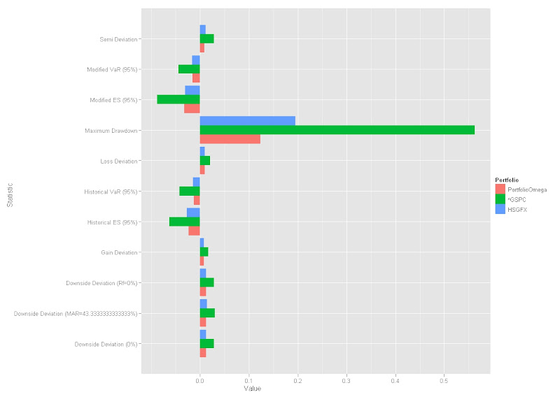
If nothing else, maybe you can use my ggplot2 chart of a PerformanceAnalytics table.  I was pretty excited to get this working, and I plan to incorporate many more of these in my testing.
From TimelyPortfolio
I blog to record my thoughts and hopefully generate a valuable dialogue with my readers who are probably far smarter and more qualified than me.  Please comment or provide feedback.
R code:
#Please see au.tra.sy blog http://www.automated-trading-system.com/
#for original walkforward/optimize code and http://www.fosstrading.com
#for other techniques
require(PerformanceAnalytics)
require(quantmod)
require(RQuantLib)
require(reshape2)  #for some fancy ggplot charting
require(ggplot2)
#get bond returns to avoid proprietary data problems
#see previous timelyportfolio blogposts for explanation
#probably need to make this a function since I will be using so much
getSymbols("GS10",src="FRED") #load US Treasury 10y from Fed Fred
GS10pricereturn<-GS10  #set this up to hold price returns
GS10pricereturn[1,1]<-0
colnames(GS10pricereturn)<-"PriceReturn"
#I know I need to vectorize this but not qualified enough yet
#Please feel free to comment to show me how to do this
for (i in 1:(NROW(GS10)-1)) {
  GS10pricereturn[i+1,1]<-FixedRateBondPriceByYield(yield=GS10[i+1,1]/100,issueDate=Sys.Date(),
    maturityDate= advance("UnitedStates/GovernmentBond", Sys.Date(), 10, 3),
    rates=GS10[i,1]/100,period=2)[1]/100-1
}
#interest return will be yield/12 for one month
GS10interestreturn<-lag(GS10,k=1)/12/100
colnames(GS10interestreturn)<-"Interest Return"
#total return will be the price return + interest return
GS10totalreturn<-GS10pricereturn+GS10interestreturn
colnames(GS10totalreturn)<-"Bond Total Return"
#get sp500 returns from FRED
getSymbols("SP500",src="FRED") #load SP500
#unfortunately cannot get substitute for proprietary CRB data
#get data series from csv file
CRB<-as.xts(read.csv("spxcrbndrbond.csv",row.names=1))[,2]
#do a little manipulation to get the data lined up on monthly basis
GS10totalreturn<-to.monthly(GS10totalreturn)[,4]
SP500<-to.monthly(SP500)[,4]
#get monthly format to yyyy-mm-dd with the first day of the month
index(SP500)<-as.Date(index(SP500))
#my CRB data is end of month; could change but more fun to do in R
CRB<-to.monthly(CRB)[,4]
index(CRB)<-as.Date(index(CRB))
#now lets merge to get asset class returns
assetROC<-na.omit(merge(ROC(SP500,type="discrete"),CRB,GS10totalreturn))
# Set Walk-Forward parameters (number of periods)
optim<-12 #1 year = 12 monthly returns
wf<-1 #walk forward 1 monthly returns
numsys<-2
# Calculate number of WF cycles
numCycles = floor((nrow(assetROC)-optim)/wf)
# Define JPT function
# this is now part of LSPM package, but fails when no negative returns
# so I still include this where I can force a negative return
jointProbTable <- function(x, n=3, FUN=median, ...) {
  # Load LSPM
  if(!require(LSPM,quietly=TRUE)) stop(warnings())
  # handle case with no negative returns
  for (sys in 1:numsys) {
    if (min(x[,sys])> -1) x[,sys][which.min(x[,sys])]<- -0.03
  }
  # Function to bin data
  quantize <- function(x, n, FUN=median, ...) {
    if(is.character(FUN)) FUN <- get(FUN)
    bins <- cut(x, n, labels=FALSE)
    res <- sapply(1:NROW(x), function(i) FUN(x[bins==bins[i]], ...))
  }
  # Allow for different values of 'n' for each system in 'x'
  if(NROW(n)==1) {
    n <- rep(n,NCOL(x))
  } else
  if(NROW(n)!=NCOL(x)) stop("invalid 'n'")
  # Bin data in 'x'
  qd <- sapply(1:NCOL(x), function(i) quantize(x[,i],n=n[i],FUN=FUN,...))
  # Aggregate probabilities
  probs <- rep(1/NROW(x),NROW(x))
  res <- aggregate(probs, by=lapply(1:NCOL(qd), function(i) qd[,i]), sum)
  # Clean up output, return lsp object
  colnames(res) <- colnames(x)
  res <- lsp(res[,1:NCOL(x)],res[,NCOL(res)])
  return(res)
}
for (i in 0:(numCycles-1)) {
            # Define cycle boundaries
            start<-1+(i*wf)
            end<-optim+(i*wf)
            # Get returns for optimization cycle and create the JPT
        # specify number of bins; does not seem to drastically affect results
        numbins<-6
            jpt <- jointProbTable(assetROC[start:end,1:numsys],n=rep(numbins,numsys))
            outcomes<-jpt[[1]]
            probs<-jpt[[2]]
            port<-lsp(outcomes,probs)
            # DEoptim parameters (see ?DEoptim)
            np=numsys*10       # 10 * number of mktsys
            imax=1000       #maximum number of iterations
            crossover=0.6       #probability of crossover
            NR <- NROW(port$f)
            DEctrl <- list(NP=np, itermax=imax, CR=crossover, trace=TRUE)
            # Optimize f
            res <- optimalf(port, control=DEctrl)
        # use upper to restrict to a level that you might feel comfortable
            #res <- optimalf(port, control=DEctrl, lower=rep(0,13), upper=rep(0.2,13))
    # these are other possibilities but I gave up after 24 hours
        #maxProbProfit from Foss Trading
        #res<-maxProbProfit(port, 1e-6, 6, probDrawdown, 0.1, DD=0.2, control=DEctrl)
        #probDrawdown from Foss Trading
        #res<-optimalf(port,probDrawdown,0.1,DD=0.2,horizon=6,control=DEctrl)
            # Save leverage amounts as optimal f
        # Examples in the book Ralph Vince Leverage Space Trading Model
        # all in dollar terms which confuses me
        # until I resolve I changed lev line to show optimal f output
        lev<-res$f[1:numsys]
            #lev<-c(res$f[1]/(-jpt$maxLoss[1]/10),res$f[2]/(-jpt$maxLoss[2]/10))
            levmat<-c(rep(1,wf)) %o% lev #so that we can multiply with the wfassetROC
            # Get the returns for the next Walk-Forward period
            wfassetROC <- assetROC[(end+1):(end+wf),1:numsys]
            wflevassetROC <- wfassetROC*levmat #apply leverage to the returns
            if (i==0) fullassetROC<-wflevassetROC else fullassetROC<-rbind(fullassetROC,wflevassetROC)
        if (i==0) levered<-levmat else levered<-rbind(levered,levmat)
}
#not super familiar with xts, but this add dates to levered
levered<-xts(levered,order.by=index(fullassetROC) )
colnames(levered)<-c("sp500 optimal f","crb optimal f")
chart.TimeSeries(levered, legend.loc="topleft", cex.legend=0.6)
#review the optimal f values
#I had to fill the window to my screen to avoid a error from R on margins
par(mfrow=c(numsys,1))
for (i in 1:numsys) {
    chart.TimeSeries(levered[,i],xlab=NULL)
}
#charts.PerformanceSummary(fullassetROC, ylog=TRUE, main="Performance Summary with Optimal f Applied as Allocation")
assetROCAnalyze<-merge(assetROC,fullassetROC)
colnames(assetROCAnalyze)<-c("sp500","crb","US10y","sp500 f","crb f")
charts.PerformanceSummary(assetROCAnalyze,ylog=TRUE,main="Performance Summary with Optimal f Applied as Allocation")
#build a portfolio with sp500 and crb
leveredadjust<-levered
#allow up to 50% allocation in CRB
leveredadjust[,2]<-ifelse(levered[,2]<0.25,0,0.5)
#allow up to 100% allocation in SP500 but portfolio constrained to 1 leverage
leveredadjust[,1]<-ifelse(levered[,1]<0.25,0,1-levered[,2])
colnames(leveredadjust)<-c("sp500 portfolio allocation","crb portfolio allocation")
assetROCadjust<-merge(assetROCAnalyze,leveredadjust[,1:2]*assetROC[,1:2])
colnames(assetROCadjust)<-c("sp500","crb","US10y","sp500 f","crb f","sp500 system component","crb system component")
charts.PerformanceSummary(assetROCadjust,ylog=TRUE)
#review the allocations versus optimal f
#I had to fill the window to my screen to avoid a error from R on margins
par(mfrow=c(numsys,1))
for (i in 1:numsys) {
    chart.TimeSeries(merge(levered[,i],leveredadjust[,i]),xlab=NULL,legend.loc="topleft",main="")
}
#add bonds when out of sp500 or crb
assetROCportfolio<-assetROCadjust[,6]+assetROCadjust[,7]+ifelse(leveredadjust[,1]+leveredadjust[,2] >= 1,0,(1-leveredadjust[,1]-leveredadjust[,2])*assetROC[,3])
assetROCadjust<-merge(assetROCAnalyze,assetROCportfolio)
colnames(assetROCadjust)<-c("sp500","crb","US10y","sp500 f","crb f","system portfolio")
charts.PerformanceSummary(assetROCadjust[,c(1:3,6)],ylog=TRUE,main="Optimal f System Portfolio with Bond Filler")
#see timelyportfolio blog post http://timelyportfolio.blogspot.com/2011/04/great-faj-article-on-statistical_6197.html
#get Correlations for Mahalanobis filter
#get data from St. Louis Federal Reserve (FRED) to add 20y USTreasury data
getSymbols("GS20",src="FRED") #load 20yTreasury; 20y has gap 86-93; 30y has gap in early 2000s
getSymbols("GS30",src="FRED") #load 30yTreasury to fill 20y gap 86-93
#fill 20y gap from discontinued 20y Treasuries with 30y
GS20["1987-01::1993-09"]<-GS30["1987-01::1993-09"]
assetROC<-merge(assetROC,momentum(GS20)/100)
corrBondsSp<-runCor(assetROC[,4],assetROC[,1],n=7)
corrBondsCrb<-runCor(assetROC[,4],assetROC[,2],n=7)
corrSpCrb<-runCor(assetROC[,2],assetROC[,1],n=7)
#composite measure of correlations between asset classes and roc-weighted correlations
assetCorr<-(corrBondsSp+corrBondsCrb+corrSpCrb+
    (corrBondsSp*corrSpCrb*assetROC[,1])+
    (corrBondsCrb*corrSpCrb*assetROC[,2])-
    assetROC[,4])/6
#sum of ROCs of asset classes
assetROCSum<-assetROC[,1]+assetROC[,2]+assetROC[,4]
#finally the turbulence measure
turbulence<-abs(assetCorr*assetROCSum*100)
colnames(turbulence)<-"Turbulence-correlation"
signal<-ifelse(turbulence>0.8,0,1)
signal<-lag(signal,k=1)
signal[0]<-0
system_perf_turbulence<-assetROCportfolio*signal
perf_compare<-merge(assetROC[,1:2],assetROCportfolio,system_perf_turbulence)
colnames(perf_compare)<-c("SP500","CRB","LSPMportfolio","LSPMportfolio_turbulence")
charts.PerformanceSummary(perf_compare,ylog=TRUE,colorset=c("gray70","goldenrod","cadetblue","darkolivegreen3"),main="Comparison of Original LSPM System and Turbulence LSPM System")
downsideTable<-melt(cbind(rownames(table.DownsideRisk(perf_compare)),table.DownsideRisk(perf_compare)))
colnames(downsideTable)<-c("Statistic","Portfolio","Value")
ggplot(downsideTable, stat="identity", aes(x=Statistic,y=Value,fill=Portfolio)) + geom_bar(position="dodge") + coord_flip()